CODE
from rdkit import Chem
from rdkit.Chem import rdChemReactions
rxn_str = "[#6:1][NX3;H2:2].[#6:3][OX2H1:4].[#6:5][OX2H1:6]>>[#6:1][N:2](CCCCCCCC(=O)[OX2H0:4][#6:3])CCCCCC(=O)[OX2H0:6][#6:5]"
rdChemReactions.ReactionFromSmarts(rxn_str)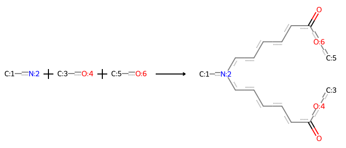
In modern AI-aided drug discovery, the chemical space addressed by the drug discovery funnel is truly vast. Virtual screening of large libraries of compounds is much higher-throughput than traditional primary screening. However, the chemical space that can be explored is still limited by the ability to enumerate and score compounds; this does not reasonably scale over many billions of compounds because of the expense of calculation on each compound, no matter how fast the calculations are.
To address this problem, we exploit the fact that we only want the highest scoring structures from a library. This is a very similar situation to online marketing or advertising matching, in which recommendations need to be made from relatively little data. There is a deep understanding of the methods that succeed in such a task. One prominent example is also one of the oldest and most versatile - Thompson sampling.
We’ll explore how Thompson sampling can be used to score chemical structures without enumerating them, and how it can be applied to the problem of virtual screening in drug discovery. For this application in chemistry, we’ll use a convenient implementation from a recent paper (Klarich et al. 2024), which is proving to be a valuable tool to exponentially amplify the power virtual of screening, by screening over fragments rather than over structures explicitly.
We continue with the recurring example of ionizable lipids in lipid nanoparticles (LNPs) for drug delivery.
The celebrated Pfizer-BioNTech and Moderna mRNA vaccines for COVID-19 use modular lipid nanoparticles (LNPs) to deliver mRNA. These formulations use different ionizable lipids, known as ALC-0315 (Pfizer-BioNTech) and SM-102 (Moderna), which are often looked upon in a modular manner:
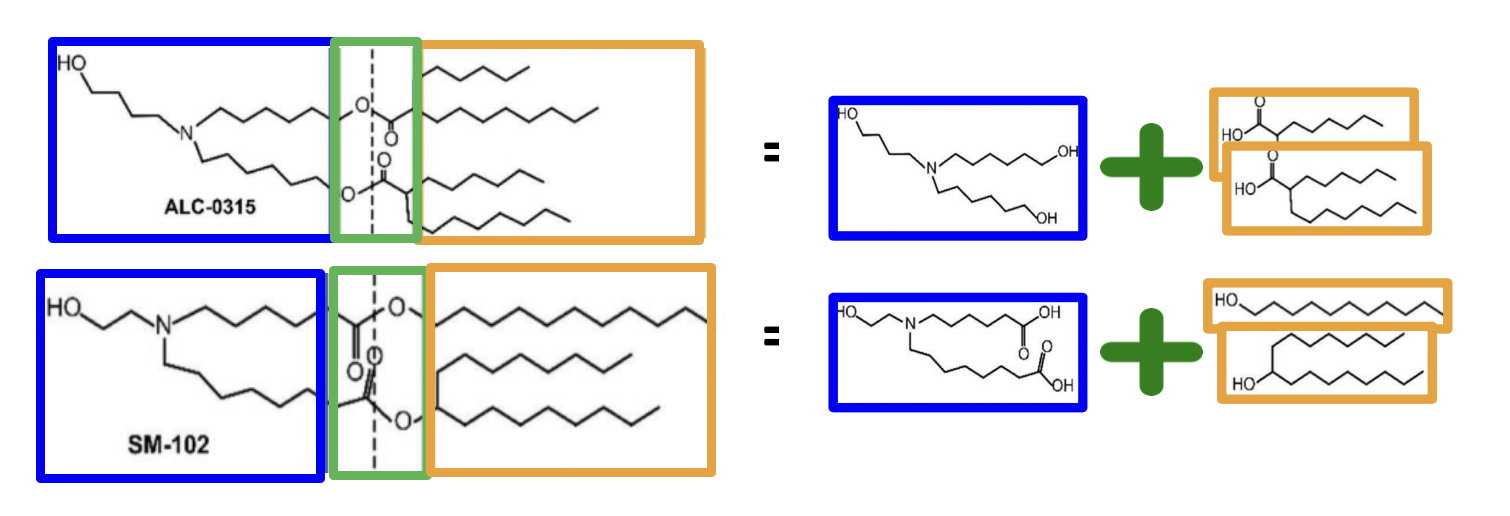
Their “reaction skeletons” are similar (ester linkages connecting two tails with some branching to a tertiary amine head group) but have important differences (e.g. their ester groups face opposite directions with respect to the head group). Suppose we want to try varying these components from one of these basic structures.
Take SM-102 as an example (for technical reasons (Zhang et al. 2023)). We might want to vary the head and tails, keeping the ester linkers intact. Let’s say we want to modify it precisely, using the large and diverse collection of hundreds of primary amine heads and hydrophobic tails outlined in previous posts. We will perform the following modifications:
Try a number of different head groups corresponding to different amines.
Keep the alkyl chain spacers separating the acid groups from the amine nitrogen (currently each tail has 5 spacer carbons before the carbonyl group).
Try different tail groups (the two alcohol-derived portions), varying the length, branching, and saturation.
LNPs are a versatile and modular technology in which the IL is formulated together with multiple (normally 3) other chemical components - they are engineered to work together to deliver the drug to its target. So the IL is not fully determinative. Such details are out of the scope of our presentation, and they may be more important for industrial-grade drug discovery efforts. However, the machine learning and tools presented here are generically useful in production-ready pipelines, and form the backbone of even more advanced engineering efforts.
To implement Thompson sampling, we need to write these modifications as a multi-component in silico “reaction” in an unambiguous way. This will have several components per the above description:
We insert the alkyl spacer carbons on either side.
from rdkit import Chem
from rdkit.Chem import rdChemReactions
rxn_str = "[#6:1][NX3;H2:2].[#6:3][OX2H1:4].[#6:5][OX2H1:6]>>[#6:1][N:2](CCCCCCCC(=O)[OX2H0:4][#6:3])CCCCCC(=O)[OX2H0:6][#6:5]"
rdChemReactions.ReactionFromSmarts(rxn_str)
Next, we gather a set of tail groups we might want to try in this variant screening. Drug designers in this field vary the tail groups in a number of ways, and we include a representative sample of these variations:
We can systematically generate a set of tail groups that vary in these ways. For virtual screening purposes, we’ll do this combinatorially, generating all possible combinations of these variations. This is discussed in more detail in another post.
In this case, the process results in thousands of candidate tail substructures.
source_pfx = "../../files/chem/"
sourcing_tools_path = source_pfx + "sourcing_ionizable_lipid_structures.py"
from importlib.machinery import SourceFileLoader
IL_structures = SourceFileLoader("IL_structures", sourcing_tools_path).load_module()from itertools import combinations, product
from rdkit import RDLogger
lg = RDLogger.logger()
lg.setLevel(RDLogger.CRITICAL) # Set the logging level to CRITICAL to suppress all messages below this level
# design‑space parameters -----------------------------------------------------
unbranched_lengths = [6, 7, 8, 9, 10, 11, 12, 13, 14, 15, 16] # carbons / tail
branched_lengths = [6, 7, 8, 9, 10, 11, 12] # carbons / tail
unsat_choices = (0, 1, 2) # number of C=C per tail
# -----------------------------------------------------------------------------
frags = set()
# unbranched tails
for L, d in product(unbranched_lengths, unsat_choices):
interior = range(1, L - 1) # keep core‑C and C‑OH single
if d > len(interior):
continue
for db in combinations(interior, d):
if not IL_structures.spacing_ok(db):
continue
try:
smi = IL_structures.build_linear_tail(L, db)
Chem.SanitizeMol(Chem.MolFromSmiles(smi))
frags.add(smi)
except:
pass # drops impossible ones silently
# ---------- branched ------------
for L1, L2, d1, d2 in product(branched_lengths, branched_lengths, unsat_choices, unsat_choices):
interior1 = range(1, L1) # skip bond 0 (core‑C1)
interior2 = range(1, L2)
if d1 > len(interior1) or d2 > len(interior2):
continue
for db1 in combinations(interior1, d1):
if not IL_structures.spacing_ok(db1):
continue
for db2 in combinations(interior2, d2):
if not IL_structures.spacing_ok(db2):
continue
try:
smi = IL_structures.build_branched_tail(L1, L2, db1, db2)
Chem.SanitizeMol(Chem.MolFromSmiles(smi))
frags.add(smi)
except Exception:
passWe can write this to a file once we’re done enumerating these moieties.
import pandas as pd
tail_pfx = "../../files/LNP_catalog/"
tail_file_path = tail_pfx + "tail_frags.smi"
names_tails = []
frags_tails = [Chem.CanonSmiles(f) for f in frags if Chem.MolFromSmiles(f) is not None]
names_tails.extend(["tail-" + str(x) for x in range(len(frags_tails))])
tails_df = pd.DataFrame([frags_tails, names_tails], index=["SMILES", "NAME"]).T
tails_df.to_csv(tail_file_path, index=False, header=False, sep=" ")
print(f"{len(frags_tails)} unique fragments written.")9892 unique fragments written.Note that this type of combinatorial expansion is much easier to do computationally than in an assay, playing to the strengths of virtual screening.
The implementation involves helper functions linear_smiles and branched_smiles, which automatically generate tails of a particular nature. When all the combinations are expanded, we have a set of many hundreds of tail groups that can be used in the screening.
import mols2grid
mols2grid.display([Chem.MolFromSmiles(x) for x in frags_tails],mol_col="mol", n_cols=7, n_rows=4)The reaction skeleton we’ve defined above involves a primary amine reactant that becomes the head group of the IL. Due to the importance of the head group to the therapeutic behavior of the IL, it is often the main focus of this screening, prompting virtual screens over a large variety of head groups.
In another post, we address exactly this issue, sourcing a large number of possible head groups. We can load the primary head groups from that post.
head_pfx = "../../files/LNP_catalog/"
old_head_df = pd.read_csv(head_pfx + "frags_amines.csv.gz", compression="gzip")
mols2grid.display([Chem.MolFromSmiles(x) for x in old_head_df["SMILES"].tolist()],mol_col="mol", n_cols=7, n_rows=4)To this, we can add a large set of primary amines from the TS implementation we are using.
import pandas as pd
amines_klarich = pd.read_csv("https://raw.githubusercontent.com/PatWalters/TS/refs/heads/main/data/primary_amines_ok.smi", header=None, sep=" ", names=["SMILES", "NAME"])
amines_klarich['N_count'] = amines_klarich['SMILES'].apply(lambda x: x.count('N') + x.count('n'))
amines_klarich = amines_klarich.sort_values(by='N_count', ascending=True)
amines_klarich = amines_klarich.drop_duplicates(subset=['SMILES'])
print("{} distinct amines from Klarich et al. 2024 library.".format(amines_klarich.shape[0]))
new_frags_heads = [Chem.CanonSmiles(x) for x in amines_klarich['SMILES']]
new_names_heads = ['_'.join(['Klarich'] + str(x).split()) for x in amines_klarich['NAME'].tolist()]
mols2grid.display([Chem.MolFromSmiles(x) for x in amines_klarich['SMILES']],mol_col="mol", n_cols=7, n_rows=4)13839 distinct amines from Klarich et al. 2024 library.This is a substantial amount of additional chemical matter for the screening, adding ~50% more fragment structures.
new_head_df = pd.DataFrame({
"SMILES": new_frags_heads,
"Name": new_names_heads
})
amine_classifications = IL_structures.summarize_amines(new_head_df["SMILES"])
new_col = {s: " | ".join(amine_classifications[s]) for s in amine_classifications}
new_head_df["Amine_type"] = new_head_df["SMILES"].map(new_col)
all_heads_df = pd.concat([old_head_df, new_head_df])
distinct_heads_df = all_heads_df.drop_duplicates(subset=["SMILES"])
print("{} head groups in the library ({} distinct head groups).".format(
all_heads_df.shape[0], distinct_heads_df.shape[0]))
distinct_heads_df.to_csv(head_pfx + "frags_amines_TS.csv.gz", compression="gzip", index=False)40261 head groups in the library (39536 distinct head groups).These modifications are sensible for the field and apply very narrowly to only the single base structure SM-102 (we could do the same for any of the hundreds of other purchasable trade lipids of interest, for instance).
But it’s easy to calculate the issue with multiple heads and tails varying simultaneously – we have made our way into a combinatorial explosion.
import numpy as np, pandas as pd
from rdkit import Chem
heads_file_path = head_pfx + "frags_amines_TS.csv.gz"
heads_df = pd.read_csv(heads_file_path, header=0, compression="gzip")
tails_df = pd.read_csv(tail_file_path, header=None, index_col=False, sep=" ", names=["SMILES", "Name"])
# Write this in scientific notation
total_size = np.prod([heads_df.shape[0], tails_df.shape[0], tails_df.shape[0]])
print(f"Total size of the design space: {total_size:.2e} structures.")Total size of the design space: 3.87e+12 structures.In a drug development pipeline, the goal is to pick “promising” structures, which typically do well in experiments and/or will determine future decisions. Since experiments are often resource-intensive and costly to perform, AI in drug development seeks to eliminate the need for testing unviable structures, and more quickly focus on promising regions of chemical space for further development. Accordingly, there are many models in drug discovery that predict everything from physicochemical properties to in vivo responses and the results of high-throughput assays.
Though these models are a poor surrogate for performing chemistry assays, their power is in being cheaply applicable to structures at will, without the need for synthesis. Chemical space is so vast, however, that we still need AI/ML methods to tell us where to turn and prospect for promising structures to experimentally test.
Methods like Thompson sampling fill in this gap, operating on top of existing models to tell us where to turn and prospect for promising structures to experimentally test. We’ll demonstrate this for ionizable lipid (IL) design in LNP development, our recurring example in other posts.
The first step in screening a chemical space is to have a model that can score the structures. For IL design, couple of notable works have made openly accessible strides in this area:
The AGILE study (Xu et al. 2024) performed combinatorial screens for an LNP with a given ionizable lipid component.
Another paper (Witten et al. 2024) has a meta-analyzed dataset of LNP activity measurements of various types from the literature, which they use to train models to guide follow-up experiments.
These are incomparable signals; not only are the studies different, but even the types of activity being measured are substantively different. Why use either of these datasets? There is value to incorporating these literature studies in an internal model, for a couple of different reasons:
We implicitly expect some common reproducible underlying phenomena driving these related studies. Identifying these in an operational way, with a model, represents real progress. Using multiple datasets allows us to compare the results and sanity-check positive controls.
LNP design is already being very inexactly modeled. The IL is not operating in situ, but rather within some highly specific environments like the endosome. The mechanism of operation depends on the cargo and other components of the formulation in imprecisely understood ways. Therefore, the models and data are not the bottleneck here, as they will not have perfect agreement anyway in industrial or clinically relevant settings.
For these reasons, we train a model on each of these datasets – the most conservative approach, which avoids losing information. We are free to use these models in a variety of ways afterward, far away from their training data - indeed, this is the underlying premise of virtual screening.
The AGILE study (Xu et al. 2024) also contains a model pretrained on their dataset; though this can be downloaded and used, we’ll train a new model on the AGILE dataset for transfection efficiency on 1200 structures.
There is significant work often put into model evaluation in published papers, but this is often not completely relevant to the part of chemical space at hand.
The main contributor to success when these models are being used is their performance at the high end of the distribution. It’s not important if they fail to achieve perfect correlation among low-scoring structures that we would never test anyway.
Here, we just train in a quick-and-dirty fashion for the above reasons since our goal is to just get a scoring function which is broadly acceptable. So we opt out of scaffold splitting or other training methods that attempt to encourage out-of-distribution generalization. These are certainly areas of further improvement in this post’s workflow.
import pandas as pd
import matplotlib.pyplot as plt
#from lightgbm import LGBMClassifier
from sklearn.ensemble import RandomForestRegressor
from sklearn.model_selection import train_test_split
from sklearn.metrics import roc_auc_score
import numpy as np
import joblib
from rdkit import Chem
from rdkit.Chem import AllChem
from rdkit.Chem import rdFingerprintGenerator
def get_FP_features(list_smiles, radius=2, nBits=2048):
"""Generate Morgan fingerprints for a list of SMILES."""
gen = rdFingerprintGenerator.GetMorganGenerator(radius=radius, fpSize=nBits)
fps = [np.array(gen.GetFingerprint(Chem.MolFromSmiles(smile))) for smile in list_smiles]
return np.vstack(fps)
agile_dataset = pd.read_csv("https://raw.githubusercontent.com/bowang-lab/AGILE/refs/heads/main/AGILE_smiles_with_value_group.csv", index_col=0)
witten_df = pd.read_csv('https://raw.githubusercontent.com/jswitten/LNP_ML/refs/heads/main/data/all_data_for_paper.csv')
witten_df = witten_df[~witten_df['smiles'].isna()]/var/folders/mn/9bz8ffcj7dj_przhmfwl3b5h0000gn/T/ipykernel_25887/1922757727.py:23: DtypeWarning: Columns (34,35,40,42,44,47,48,49,53,54,55,57) have mixed types. Specify dtype option on import or set low_memory=False.
witten_df = pd.read_csv('https://raw.githubusercontent.com/jswitten/LNP_ML/refs/heads/main/data/all_data_for_paper.csv')agile_fps = get_FP_features(agile_dataset['combined_mol_SMILES'].tolist())
X_train, X_test, y_train, y_test = train_test_split(agile_fps, agile_dataset['expt_Hela'])
rgr = RandomForestRegressor()
rgr.fit(X_train, y_train)
level = rgr.predict(X_test)
metric = np.sqrt(((level - y_test)** 2).mean())#rgr.score(X_test, y_test)
plt.scatter(y_test, level)
plt.xlabel('Experimental Hela IC50')
plt.ylabel('Predicted Hela IC50')
plt.title(f'Regressor RMSE on AGILE Dataset: {metric:.3f}')
# Draw a diagonal line, and a best fit line
ymin, ymax = y_test.min()-1, y_test.max()+1
plt.plot([ymin, ymax], [ymin, ymax], 'k--', lw=2, color='red')
plt.xlim(ymin, ymax)
plt.ylim(ymin, ymax)
plt.gca().set_aspect('equal', adjustable='box')
plt.grid()
plt.tight_layout()
#plt.savefig('agile_regressor_performance.png', dpi=300)
plt.show()/var/folders/mn/9bz8ffcj7dj_przhmfwl3b5h0000gn/T/ipykernel_25887/1646678954.py:14: UserWarning: color is redundantly defined by the 'color' keyword argument and the fmt string "k--" (-> color='k'). The keyword argument will take precedence.
plt.plot([ymin, ymax], [ymin, ymax], 'k--', lw=2, color='red')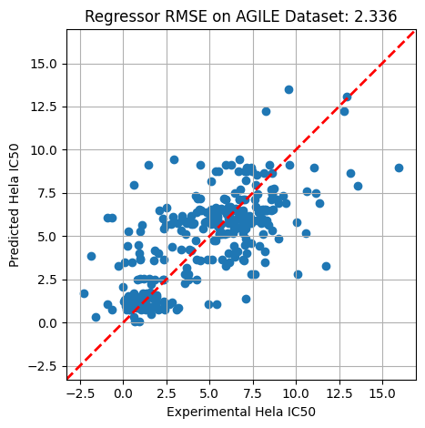
Now we can train a regressor on the full AGILE dataset, and save it.
rgr = RandomForestRegressor()
rgr.fit(agile_fps, agile_dataset['expt_Hela'])
pfx_models = '../../files/LNP_catalog/'
joblib.dump(rgr, pfx_models + 'model_agile_Hela.pkl')
# rgr = joblib.load(pfx_models + 'model_agile_Hela.pkl')['../../files/model_agile_Hela.pkl']The same can be done for the Witten et al. dataset.
witten_fps = get_FP_features(witten_df['smiles'].tolist())
X_train, X_test, y_train, y_test = train_test_split(witten_fps, witten_df['quantified_delivery'])
rgr = RandomForestRegressor()
rgr.fit(X_train, y_train)
level = rgr.predict(X_test)
metric = np.sqrt(((level - y_test)** 2).mean())#rgr.score(X_test, y_test)
# Get pearson correlation
from scipy.stats import pearsonr
corr, _ = pearsonr(level, y_test)
print(f'Pearson correlation: {corr:.3f}')
plt.scatter(y_test, level)
plt.xlabel('Experimental value')
plt.ylabel('Predicted value')
plt.title(f'Pearson correlation on Witten et al. Dataset: {corr:.3f}')
# Draw a diagonal line, and a best fit line
ymin, ymax = y_test.min()-1, y_test.max()+1
plt.plot([ymin, ymax], [ymin, ymax], 'k--', lw=2, color='red')
plt.xlim(ymin, ymax)
plt.ylim(ymin, ymax)
plt.gca().set_aspect('equal', adjustable='box')
plt.grid()
plt.tight_layout()
#plt.savefig('agile_regressor_performance.png', dpi=300)
plt.show()Pearson correlation: 0.542/var/folders/mn/9bz8ffcj7dj_przhmfwl3b5h0000gn/T/ipykernel_25887/1307831851.py:19: UserWarning: color is redundantly defined by the 'color' keyword argument and the fmt string "k--" (-> color='k'). The keyword argument will take precedence.
plt.plot([ymin, ymax], [ymin, ymax], 'k--', lw=2, color='red')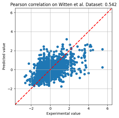
The original paper (Witten et al. 2024) does not provide evaluation on the whole dataset, but rather on the more appropriate setting of individual experiments. For ease of comparison, we evaluate the same metric as the paper on individual experiments below.
import matplotlib.pyplot as plt
# ---- prep --------------------------------------------------------------
grouped = witten_df.groupby("Experiment_ID")
n_groups = len(grouped) # should be 16, but works for any n ≤ 16
n_cols = 4
n_rows = int(np.ceil(n_groups / n_cols))
# global limits so the identity line lines up across panels
all_vals = witten_df["quantified_delivery"].values
global_min = all_vals.min() - 1
global_max = all_vals.max() + 1
fig, axes = plt.subplots(n_rows, n_cols,
figsize=(n_cols*4, n_rows*4),
sharex=False, sharey=False)
axes = axes.flatten() # easier indexing
# ---- plot each group ---------------------------------------------------
for ax, (exp_id, group) in zip(axes, grouped):
y_true = group["quantified_delivery"].values
y_pred = rgr.predict(get_FP_features(group["smiles"].tolist()))
r, _ = pearsonr(y_pred, y_true)
ax.scatter(y_true, y_pred, alpha=0.7)
ax.plot([global_min, global_max], [global_min, global_max],
ls="--", lw=2, color="red")
ax.set_xlim(global_min, global_max)
ax.set_ylim(global_min, global_max)
ax.set_aspect("equal", adjustable="box")
ax.set_title(f"ID {exp_id}\nPearson corr. = {r:.3f}")
ax.grid()
# ---- tidy up -----------------------------------------------------------
for ax in axes[n_groups:]: # hide any unused panels
ax.axis("off")
fig.tight_layout()
plt.show()/var/folders/mn/9bz8ffcj7dj_przhmfwl3b5h0000gn/T/ipykernel_25887/862537745.py:24: ConstantInputWarning: An input array is constant; the correlation coefficient is not defined.
r, _ = pearsonr(y_pred, y_true)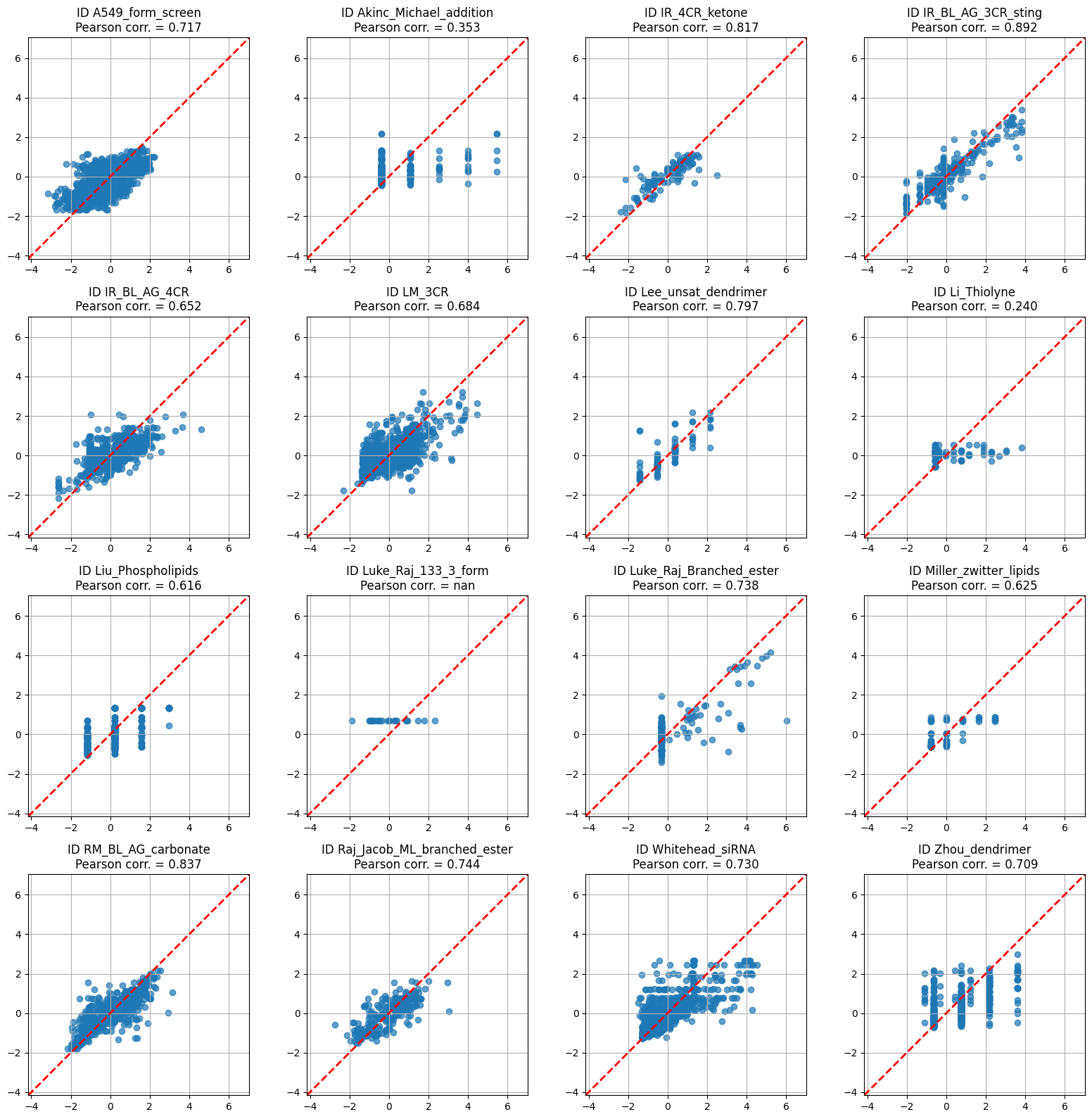
We use the Pearson correlation coefficient \(r\) here to ease comparison of this assessment to the original paper’s, where under these conditions the authors trained a more computationally intensive and accurate deep model. Our model is competitive with the original (\(r \gtrsim 0.6\) on most groups), and the performance on most groups is even better than the overall average. The performance is not perfect – the experimental values here are z-scores – but we proceed with this model as being a similarly good starting point to its published counterpart.
Again, we save the model for later scoring purposes.
rgr = RandomForestRegressor()
rgr.fit(witten_fps, witten_df['quantified_delivery'])
pfx_models = '../../files/LNP_catalog/'
joblib.dump(rgr, pfx_models + 'model_witten.pkl')
# rgr = joblib.load(pfx_models + 'model_witten.pkl')['../../files/LNP_catalog/model_witten.pkl']Thompson sampling (TS) is a decision-making method used to efficiently learn which option is best when facing uncertain outcomes. It was originally developed in the context of clinical trials, and is now widely used in machine learning and experimental design. It balances two paradigmatic goals in tension:
Exploration: Testing uncertain or less-studied compounds to improve overall knowledge.
Exploitation: Focusing on compounds already showing promise to efficiently optimize outcomes.
Thompson sampling works with a distribution over experimental outcomes representing the scientist’s current beliefs. At any point in time, these beliefs can be sampled to suggest a best course of action (e.g. compounds to test next). Thompson sampling consists of taking this action and updating the belief distribution according to Bayes’ rule.
It is well-understood, both empirically and theoretically, that such a strategy can work even if the initial belief distribution is dramatically misspecified. As more data is collected, the belief distribution converges to the true distribution of outcomes, and the sampling strategy becomes more focused on the options that are truly best.
A typical experimental context involves screening compounds to identify which yield the highest activity. Initially the experimentalist has little information, and belief distributions have high uncertainty, so Thompson sampling often samples high values even for options with lower estimated means, encouraging exploration. If a compound performs well, the experimentalist’s belief in its future performance shifts upward, increasing the likelihood that future samples will lead to selecting it again. Conversely, poor performance lowers future expectations. Over time, this naturally guides experiments toward the most promising compounds, while still periodically exploring less-understood ones to confirm or revise the current understanding. Eventually, the uncertainty ceases to dominate, and sampling tends to favor options with better estimated outcomes.
This approach elegantly and naturally balances exploration and exploitation, analogous to how method development is often approached anyway —- initially trying diverse approaches before refining the most promising ones.
The TS algorithm is one of the workhorses of modern machine learning. The trick is often in how well it works in practice, and here we try it on the truly vast library of ionizable lipids from the literature put together above. In this post, we’ll construct such a library and perform this virtual scoring effort in a realistic lipid nanoparticle engineering context. This is paradigmatic of many small molecule drug discovery subfields, but with a combination of very broad application and a truly vast design space.
import joblib
pfx_models = '../../files/LNP_catalog/'
rgr_agile = joblib.load(pfx_models + 'model_agile_Hela.pkl')
rgr_witten = joblib.load(pfx_models + 'model_witten.pkl')To finish setting up the TS algorithm, we need to precisely define the scoring function that will be used to evaluate the structures. This implementation constrains us to implement the evaluator as a separate class in its evaluators.py file. Crucially, we include the same fingerprint extraction function that was used to featurize the compounds for training.
class NewMLModelEvaluator(Evaluator):
def __init__(self, input_dict):
self.mdl = joblib.load(input_dict["model_filename"])
self.num_evaluations = 0
@property
def counter(self):
return self.num_evaluations
def _get_FP_features(list_smiles, radius=2, nBits=2048):
"""Generate Morgan fingerprints for a list of SMILES."""
gen = rdFingerprintGenerator.GetMorganGenerator(radius=radius, fpSize=nBits)
fps = [np.array(gen.GetFingerprint(Chem.MolFromSmiles(smile))) for smile in list_smiles]
return np.vstack(fps)
def evaluate(self, mol):
self.num_evaluations += 1
return self.mdl.predict(_get_FP_features([Chem.MolToSmiles(mol)]))The above code should be added to the evaluators.py file in the TS working directory.
Finally, all this gets put together in the config file for the TS algorithm, which specifies the reaction schema and scoring function to use. The reagent files are assumed to be plaintext two-column space-separated files, with the first column being the SMILES and the second column being the name of the reagent. We ensure that our compressed files of fragment libraries are rewritten in this format.
import pandas as pd
import gzip
# Read ../../files/frags_amines_TS.csv.gz, unzip it and write it to ../../files/frags_amines_TS.smi
df = pd.read_csv(pfx + 'frags_amines_TS.csv.gz', compression='gzip')
df.iloc[:, :2].to_csv(pfx + 'frags_amines_TS.smi', index=False, header=False, sep=" ")head_file_path = pfx + "frags_amines_TS.smi"
tail_file_path = pfx + "tail_frags.smi"
model_path = pfx_models + "model_witten.pkl" # Change to ../../files/model_agile.pkl as necessary
# Already defined above
# rxn_str = "[#6:1][NX3;H2:2].[#6:3][OX2H1:4].[#6:5][OX2H1:6]>>[#6:1][N:2](CCCCCCCC(=O)[OX2H0:4][#6:3])CCCCCC(=O)[OX2H0:6][#6:5]"
config_dict = {
"reagent_file_list": [
head_file_path,
tail_file_path,
tail_file_path
],
"reaction_smarts": rxn_str,
"num_warmup_trials": 10,
"num_ts_iterations": 10000,
"evaluator_class_name": "NewMLModelEvaluator",
"evaluator_arg": {
"model_filename": model_path
},
"ts_mode": "maximize",
"log_filename": "ts_logs.txt",
"results_filename": pfx + "classification_model_out.csv"
}
json_file_path = pfx + "TS_example_LNP.json"
# Write config_dict to a json file
import json
with open(json_file_path, 'w') as f:
json.dump(config_dict, f, indent=4) # indent for pretty-printing
# Example: Reading from a file
with open(json_file_path, 'r') as f:
data = json.load(f)
data{'reagent_file_list': ['../../files/LNP_catalog/frags_amines_TS.smi',
'../../files/LNP_catalog/tail_frags.smi',
'../../files/LNP_catalog/tail_frags.smi'],
'reaction_smarts': '[#6:1][NX3;H2:2].[#6:3][OX2H1:4].[#6:5][OX2H1:6]>>[#6:1][N:2](CCCCCCCC(=O)[OX2H0:4][#6:3])CCCCCC(=O)[OX2H0:6][#6:5]',
'num_warmup_trials': 10,
'num_ts_iterations': 10000,
'evaluator_class_name': 'NewMLModelEvaluator',
'evaluator_arg': {'model_filename': '../../files/LNP_catalog/model_witten.pkl'},
'ts_mode': 'maximize',
'log_filename': 'ts_logs.txt',
'results_filename': '../../files/LNP_catalog/classification_model_out.csv'}import pandas as pd
import useful_rdkit_utils as uru
#from lightgbm import LGBMClassifier
from sklearn.ensemble import RandomForestRegressor
from sklearn.model_selection import train_test_split
from sklearn.metrics import roc_auc_score
import numpy as np
import joblib
from rdkit import Chem
from rdkit.Chem import AllChem
from rdkit.Chem import rdMolDescriptors
import evaluators as evl
def predict_with_model(
smiles,
model_filename
):
model = joblib.load(model_filename)
#fp = np.array(rdMolDescriptors.GetMorganFingerprintAsBitVect(Chem.MolFromSmiles(smiles), 3, nBits=2048))
return model.predict(evl.get_FP_features([smiles]))
predict_with_model('CC', pfx_models + 'model_witten.pkl')Thompson sampling is now run, and the sequence of computations is a useful way to look at what we have gained here. The theme is processing in a way that scales mainly with the number of fragments, and less so with the combinatorics.
There is an initial “warm-up” phase in which each fragment is sampled in the context of a random structure or two to get a baseline for that fragment’s typical score.
Then, the TS algorithm is run for a fixed number of iterations, with each iteration sampling a new structure. This is the main part of the computation in which the sampling gradually hill-climbs towards high-scoring structures. In fairly few iterations, it typically finds plateaus of high-scoring structures; for virtual screening applications guided by data-poor models, this is basically the best an optimization method can do.
The warm-up phase only scales in the number of fragments. The sampling phase then typically only requires a relatively small few thousand fixed number of iterations to find good plateaus in the model scoring function.
When the TS algorithm is run with the above config file in the repository’s local directory, the results look like this:
import importlib
from ts_main import read_input, run_ts
ts_input_dict = read_input('TS_example_LNP.json')
score_df = run_ts(ts_input_dict)score_df.to_csv(pfx + 'model_witten_scores.csv', index=False)import pandas as pd
score_df = pd.read_csv(pfx + 'model_witten_scores.csv')
score_dfimport numpy as np
a = [x.split('_tail')[0] for x in score_df['Name']]
asrt = np.unique(a, return_counts=True)
head_smiles = dict(zip(
asrt[0][np.argsort(asrt[1])[::-1]],
asrt[1][np.argsort(asrt[1])[::-1]]
))
head_smilesSince the model does not give enough guidance to optimize further beyond the plateaus it finds, the structures it generates are severely under-determined. It could easily generate other structures in a given run, but the sets of structures it generates each run will have similar scores, and possibly be structurally similar to each other.
Exploring these plateaus must be done by other means. We can get a sense at least for how to expand combinatorially around a given structure by varying each of its fragments systematically in a sensible neighborhood-aware way.
This type of post-processing naturally overlaps with filtering steps that are essential in any given drug program in order to conform with program-specific real-world constraints.
The scoring can be done in a quite flexible way, to incorporate all manner of criteria. Here are a few examples:
General objective functions: Thompson sampling as an approach only maximizes functions, but this is completely general. If we are looking to be in a particular region, for example,
Multi-objective optimization: We can optimize for multiple criteria at once. This is a very powerful approach in drug discovery in particular, where high-stakes, inexact decisions are constantly made with incomplete scientific information. Another post discusses this in more detail.
Normalization of each dataset can be done relative to predictions in that dataset. Taking the prediction percentile in a particular dataset is an easy primitive that can be aggregated across different datasets to give weighted normalized rankings of various kinds. It turns out that these are incredibly powerful in practice, as they correspond to only searching over particularly highly ranked predictions.
Taken together, these forms a fully general toolkit for efficiently, easily, and interpretably dealing with multi-criteria and decision making.
@online{balsubramani,
author = {Balsubramani, Akshay},
title = {Screening Too Many Chemicals to Count},
langid = {en}
}