To many in sports or other fields of competition, the problem of determining a global ranking of competitors or teams from a sparse collection of one-on-one matches is a familiar one. This problem has arisen in competitive endeavors like in soccer, tennis, or chess, as well as LLM evaluation mechanisms. there are systems of doing this which can be strange and opaque to varying degrees, but ultimately come up with a “reasonable” ranking.
This post is about one such method – a beautiful and efficient application of linear algebra, which is widely known in some disciplines and revelatory in others. It relies on a collection of tools for calculus – measuring local change – on graphs.
Measuring change on graphs
It consists of tools which are embarrassingly simple to implement, but Python toolboxes that implement these tools often don’t expose or document them in a way that’s readily broken down and understood. Here we’ll develop this “graph calculus,” and implement it efficiently.
The graph could represent a manifold, about which much has been written elsewhere; graph calculus is a powerful toolbox to efficiently and nonparametrically manipulate functions on these manifolds, mimicking the original inventions of these calculus tools to model physics phenomena.
Getting global rankings from matches
There’s a very neat way to conceptualize the problem of getting a global ranking from pairwise comparisons. It relies on two steps: making a graph out of the matches played, and then computing a unique global ranking on this graph.
Making a graph from match results
Suppose we have results from a number of one-on-one matches between a group of players. If we draw these players as nodes, we can connect them with edges - one for each match, pointing from losers to winners.
This is a (directed) graph! If we’re required to rank the players, we’d like higher-ranked players to beat lower ones. For many input graphs, there might not be a ranking that perfectly satisfies this, but we’d at least want results to agree with rankings in most matches, most of the time, and more often for a bigger ranking gap. We’d generally consider any ranking that does this to be “reasonable” given the match result graph.
We can calculate a “reasonable” ranking of points for any match results, such that the match results largely follow these rankings as much as possible.
Ranking graph nodes
To do this, we rely on a linear-algebra framework that was first discovered by physicists and is now touched on in undergraduate vector calculus classes. This is laid out in the next section “Formulating a graph calculus”. That can be skipped if you aren’t interested in the details and derivation, and can be read standalone.
After that, the section “Global rankings from the graph” contains the recipe for computing a “potential function” over nodes, from which the ranking is easily computed.
Finally, the last section contains experiments before a summary.
Formulating a graph calculus
Consider an undirected connected weighted graph on \(n\) vertices represented by a symmetric adjacency matrix \(K \in \mathbb{R}^{n \times n}\). This stands in for a manifold. From a data science perspective, we can think of this in a couple of ways:
As a binary (0-1) matrix where \(K (x, y) = 1\) iff \(x\) and \(y\) have a bilateral symmetric relationship defined between them (e.g. they have played a match).
As a neighborhood graph, where \(K (x, y) = 0\) unless \(x\) and \(y\) are nearby neighbors.
On this graph \(K\), there are analogues of scalar and vector fields from multivariate calculus:
Scalar field - represented by a function on the graph vertices: a vector \(g \in \mathbb{R}^{n}\).
Vector field - represented by a function on the graph edges: a matrix \(G \in \mathbb{R}^{n \times n}\).
Definitions of graph calculus
The gradient of a scalar field \(g\) is a vector field \(\nabla g\) connecting neighboring vertices in \(K\) by their differences: \[ [\nabla g] (x, y) := ( g (x) - g (y) ) \cdot \textbf{1} (K (x, y) \> 0) \]
It is a natural way to represent changes in a function over the manifold.
Flows
A vertex \(x\) has degree \(d (x) = \sum_{y} K (x, y)\); define \(D := \text{diag} (d)\) to be the diagonal matrix constructed from \(d\). Any vector field \(G\) has a symmetric part \(\textsf{sym}\;G\), with \([\textsf{sym}\;G] (x, y) = \frac{1}{2} (G (x, y) + G (y, x))\).
The field \(G\) is called antisymmetric if \(\textsf{sym}\;(G) = 0\). Such a field is also called a flow – the prototypical example is the gradient flow \(G := \nabla g\).
CODE
import sys, numpy as np, time, scipy, scipy.linalgimport os, sklearnimport matplotlib.pyplot as plt%matplotlib inlineimport anndata, scanpy as scdef symmetric_part(A):""" Returns the symmetrized version of the input matrix. """return0.5*(A + A.T)def asymmetric_part(A):""" Returns the anti-symmetrized version of the input matrix. """return0.5*(A - A.T)def grad_op_graph(fn, adj_mat):""" Gradient of a function on a (n x n) graph. Args: fn: A function on vertices (n-dimensional vector) adj_mat: (n x n) Adjacency matrix of graph Returns: Matrix ((n x n) directed graph) of gradients on edges. """return adj_mat.multiply(fn) - adj_mat.multiply(fn).T
Differential operators
Given a vector field \(G\), the divergence of \(G\) is a scalar field measuring the net flux of signal leaving each vertex.
The curl of \(G\) is a vector field that’s basically a symmetrized version of G’s local magnitude along an edge. \[
[\textsf{curl}\; G] (x, y) := \frac{\textbf{1} (K (x, y) \> 0) }{2
K (x, y)} (G (x, y) + G (y, x)) \]
Second derivatives: the Laplacian
With these differential operators defined, we can write some properties of second derivatives that correspond to their analogues in vector calculus. Importantly, we define the Laplacian of \(G\).
\[
[\nabla^2 g] (x) := \text{scalar Laplacian of G} = [\textsf{div}
(\nabla g )] (x) = g(x) - \frac{1}{d(x)} \sum_{y \neq x} K (x, y)
g(y) = (I - D^{-1} K) g \]
There are many other normalizations of the Laplacian, but this is the one that’s most naturally interpretable for our purposes. The definition of the operators also makes clear that \(\textsf{div} (\textsf{curl}\; G) = 0\), exactly as in vector calculus. Similarly, \(\textsf{curl} (\nabla g) = 0\) as well.
CODE
def compute_transitions_asym(adj_mat): W = symmetric_part(adj_mat) recip = np.reciprocal(np.asarray(W.sum(axis=0)).astype(np.float64)) recip[np.isinf(recip)] =0return scipy.sparse.spdiags(recip, 0, W.shape[0], W.shape[0]).dot(W)def laplacian_op_graph(adj_mat, normalize=True):""" Laplacian of a function over graph vertices. Args: adj_mat: adjacency matrix for data kNN graph. normalize: Whether to degree-normalize the Laplacian matrix. Returns: Laplacian matrix (V x V). """ifnot normalize: lapmat = scipy.sparse.diags(np.ravel(adj_mat.sum(axis=0))) - adj_matelse: lapmat = scipy.sparse.identity(adj_mat.shape[0]) - compute_transitions_asym(adj_mat)return lapmatdef div_op_graph(field_mat, adj_mat):""" Divergence of a function in a neighborhood on the data manifold. Args: field_mat: a vector field (function on edges, i.e. (V x V) matrix-valued) adj_mat: adjacency matrix for data kNN graph. Returns: Array of vertex-wise divergence values. """ trans_mat = compute_transitions_asym(adj_mat)return np.ravel(trans_mat.multiply(asymmetric_part(field_mat)).sum(axis=1))def curl_op_graph(field_mat, adj_mat):""" Curl of a function on edges of a (cell x cell) graph. Args: field_mat: a vector field (function on edges, i.e. (V x V) matrix-valued) adj_mat: (cell x cell) Adjacency matrix of graph Returns: Matrix of curl associated with each edge. """ np.reciprocal(adj_mat.data, out=adj_mat.data)return adj_mat.multiply(symmetric_part(field_mat))
Connections to physics and the fundamental theorem
These notions are very familiar to physicists. In fact, all of them – the divergence, curl, and Laplacian – were invented to quantitatively describe physics phenomena, and later became part of vector calculus. They are now central to continuous ways of describing the physical world, as in Maxwell’s equations of electrodynamics, fluid mechanics, and relativity. Maxwell’s equations in particular have strong roots in the fundamental theorems of vector calculus describing divergence, flux, and integration by parts.
To tie all this together mathematically, we can prove a fundamental theorem of graph calculus that deals with the relationship between a signal’s Laplacian in a region and its flux exiting the region.
For any functions \(g, h\) on vertices and a non-empty subset \(\Omega \subseteq V\),
The term \(\sum_{x \in \Omega} \sum_{y
\in \Omega} K (x, y) (g(x) - g(y)) h(x)\) can also be written as \(\sum_{y \in \Omega} \sum_{x \in
\Omega} K (y, x) (g(y) - g(x)) h(y)\), interchanging the roles of \(x\) and \(y\). Since \(K\) is symmetric, averaging these two expressions gives \(\frac{1}{2} \sum_{x
\in \Omega} \sum_{y \in \Omega} K (x, y) (g(x) - g(y)) (h(x) -
h(y))\). Thus we deduce that
Substituting this in the equation \((*)\) above gives the result.
Special cases
As special cases, we can get fundamental forms of Gauss’s law (the divergence theorem) describing flux and the Laplacian, and Green’s identities describing integration by parts:
\(\textbf{Green's identities}\)
For any functions \(g, h\) on vertices,
\[ \begin{aligned} \sum_{x
\in \Omega} \nabla^2 g(x) d(x) &= - \sum_{x \in \Omega} d(x)
\sum_{ y \in \Omega^c} [\nabla g] (x, y) \frac{K (x, y)}{d(x)}
\;\;\forall \Omega \subseteq V \qquad &(\text{Gauss's Law}) \\
\sum_{x \in V} h (x) \nabla^2 g (x) d(x) &= \frac{1}{2} \sum_{x,
y \in V} [\nabla g] (x, y) [\nabla h] (x, y) K (x, y) \qquad
&(\text{First Green's identity}) \\ \sum_{x \in V} h (x) \nabla^2
g (x) d(x) &= \sum_{x \in V} g (x) \nabla^2 h (x) d(x) \qquad
&(\text{Second Green's identity}) \end{aligned} \]
\(\textbf{Other second derivatives on the
graph}\)
\[ [\Delta G] (x, y) := \text{vector
Laplacian of G} = [\textsf{curl} (\textsf{curl}\; G) - \nabla
(\textsf{div}\; G ) ] (x, y) = \frac{1}{2 K (x, y)^2} (G (x, y) + G
(y, x)) - \left[ \nabla (\textsf{div}\; G ) \right] (x, y)
\]
Interpreting the calculus
Just as in the standard vector calculus, these are all linear operators. They’re completely local, and interact nicely with each other and complementarily to the “Fourier basis” on the graph (the eigenbasis of the Laplacian) used for so much spectral learning.
A note on normalization and defining this calculus
This task of writing up the calculus involves more detailed choices than may first appear. There are a couple of different normalizations of the Laplacian, corresponding to different ways of calculating the divergence and gradient.
We are choosing the “non-self-adjoint” way to write this, which is less symmetric mathematically; but it is preferred here for the nice interpretations it gives divergences and gradients.
To be specific, we can define inner products on the vertices and edges of the graph.
\[ \langle a, b
\rangle_{V} = \sum_x a(x) b(x) d(x) \qquad \qquad \langle A, B
\rangle_{E} = \sum_{(x, y) \sim e} A(x, y) B(x, y) K (x, y)
\]
Having defined this, the divergence is defined to be the “adjoint” of the gradient, satisfying the following equation for any functions \(f\) over vertices and \(G\) over edges:
\[ - \langle f, \textsf{div}\; G \rangle_{V} = \langle \nabla f, G \rangle_{E} \]
In physics and math, a fundamental result of vector calculus is that the divergence and curl operators, used to model fluids locally, can be used to decompose any vector field. (This power is why Maxwell’s equations completely describe any electromagnetic field.) The resulting scalar and vector potentials are wonderful ways to understand the local behavior of these fluids. We can show the same result for functions on graphs!
This is the Helmholtz decomposition(Lim 2020): any function over edges \(G\) can be decomposed as \[ G = - \nabla \Phi + U +
S \]
where
\(\Phi\) is a vertex potential function (with \(\textsf{curl} (\nabla \Phi) = 0\))
\(S\) is a symmetric edge potential function that is closest to \(G\), i.e. minimizes \(\|\| S - G \|\|\)
\(U\) is a harmonic (globally conservative) function on edges with \(\textsf{div} ( U) = 0\) and \(\textsf{curl} ( U) = 0\)
Given the above properties, all these functions are unique (\(\Phi\) up to constant shift) and efficiently calculable:
where \((\nabla^2)^{+}\) is the pseudoinverse of the Laplacian \(\nabla^2\).
CODE
def helmholtz( field_mat, adj_mat, given_divergence=None):""" Compute Helmholtz decomposition of input edge function on graph. Args: adj_mat: adjacency matrix for data kNN graph. field_mat: a vector field (function over edges, i.e. matrix-valued) given_divergence: a given divergence function over vertices. Replaces the use of field_mat if the source/sink info is known. Returns: Pair of (vertex potential P, edge potential S) such that field_mat = - ∇P + S + U where U is a "harmonic" edge flow which is divergence-free, and 0 when field_mat is symmetric. """ laplacian_op = laplacian_op_graph(adj_mat)if given_divergence isnotNone: sympart = scipy.sparse.csr_matrix(adj_mat.shape) potential = scipy.sparse.linalg.lsmr( laplacian_op, given_divergence )else: sympart = symmetric_part(field_mat) potential = scipy.sparse.linalg.lsmr( laplacian_op, div_op_graph(field_mat, adj_mat) )return (potential[0], sympart)
In words, any function on edges \(G\) can be broken up into:
A gradient flow \(- \nabla \Phi\) that is globally acyclic (curl-free)
A curl flow \(S\) that is locally cyclic (div-free)
A harmonic flow \(U\) that is locally cyclic but globally acyclic (div-free and curl-free)
This translates to our graph manifold a cornerstone theorem of fluid dynamics (Chorin and Marsden 1990).
Proof of decomposition
This section can be skipped without loss of meaning - it has a proof of the decomposition.
First, take \(S = \frac{1}{2} (G + G^{\top})\), which possesses the desired properties, since it is the unique projection of \(G\) on to symmetric matrices (Fan and Hoffman 1955). This leaves the anti-symmetric edge vector \(F = G - S\), which can further be decomposed by a lemma.
\(\textbf{Lemma. }\) For any anti-symmetric edge vector \(F\), there is a unique function \(\Phi\) (up to constant shift) on vertices, and a unique function \(U\) on edges with \(\textsf{div} ( U) = 0\) and \(\textsf{curl} ( U) = 0\), such that \[ F = - \nabla \Phi + U \] Also, \(\Phi\) can be directly calculated: \(\Phi = (\nabla^2)^{+}
(\textsf{div}\; F)\).
\(\textbf{Proof of lemma}\)
First note that since \(\textsf{curl} (\nabla \Phi) = 0\), \(\textsf{curl} ( U) = \textsf{curl} ( F) = 0\) since \(F\) is anti-symmetric.
To show uniqueness of \(\Phi\) up to shift, assume that \(\Phi\) and \(\Phi_2\) are two functions on vertices with properties as defined in the lemma statement. Since \(\textsf{div}\;U = 0\) by assumption, we have
By similar reasoning, \(\displaystyle \textsf{div}\; F = \nabla^2 \Phi_2\).
It can be verified that since the graph is connected, \(\nabla^2\) has a one-dimensional null space (eigenvalue \(0\)), spanned by the corresponding eigenvector \(\textbf{1}\), the all-ones vector. So \(\nabla^2 \Phi = \nabla^2 \Phi_2 \iff \nabla^2 (\Phi - \Phi_2 ) = 0 \iff \Phi - \Phi_2 = c \textbf{1}\) for some constant \(c\), proving that \(\Phi\) is unique up to constant shift.
This defines a unique \(\nabla \Phi\), showing that \(U = F + \nabla \Phi\) is unique in the decomposition given \(F\).
This also shows that \(\nabla^2\) is of full rank orthogonal to the one-dimensional subspace spanned by \(\textbf{1}\), so that we can recover \(\Phi = (\nabla^2)^{+} (\textsf{div}\; F)\) up to constant shift.
This concludes the proof.
Given the lemma, the rest of the decomposition follows by noting that:
\(\textsf{div}\; S = 0\) since \(S\) is symmetric, so \(\textsf{div}\; F = \textsf{div}\; G\), so \(\Phi = (\nabla^2)^{+} (\textsf{div}\; G)\).
For a given \(G\), \(S\) is unique, so \(F\) is unique, so by the lemma, \(\Phi\) and \(U\) are unique.
Interpreting the decomposition
We can show that the potential \(\Phi\) solves a corresponding least-squares problem, finding the function whose gradient best approximates \(G\):
\[ \min_{\Phi} \frac{1}{2} \left\| \nabla \Phi - G \right\|^2 \]
We are often looking for a part of the flow that is the gradient of some potential function. The symmetric part of the flow \(S\) can therefore be ruled out immediately as having no part to play in any gradient.
This leaves the anti-symmetric part \(F := \nabla \Phi + U\). We have shown that \(U\) is the divergence-free part of \(F\), which is cyclic flow without sources/sinks. Meanwhile, the source/sink-induced component of \(F\) is the gradient flow \(\nabla \Phi\).
This decomposition is a very general fact; the potential it produces has a relationship to social choice theory as well, generalizing foundational Borda and Kemeny ranking methods (Jiang et al. 2011).
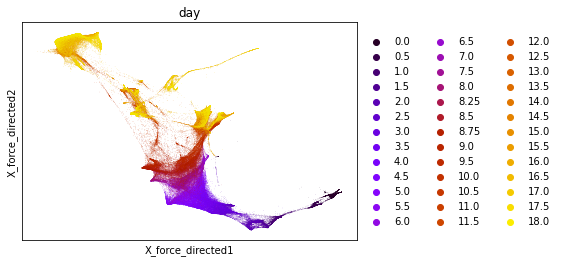
Interpolating reprogramming potential from fibroblasts to final cell fates
In biology and in particular the measurement of cell populations, this has major links to the famous developmental biologist Waddington’s idea of a “developmental landscape”. This was introduced to express the idea that cell state transitions are essentially low-dimensional phenomena occurring among a high-dimensional context of many genes, proteins, and other biomolecules. So all these biochemical changes occur in a coordinated fashion to push cells from one low-dimensional state to another, which Waddington conceptualized balls rolling “down” the landscape of “developmental potential.” This qualitative idea has had many quantitative realizations, and bears an interesting relationship to the very quantifiable Helmholtz scalar potential.
This can be demonstrated using a landmark single-cell RNA-seq dataset that reprogrammed mouse fibroblasts to stem cells (Schiebinger et al. 2019), obtainable from the CellRank package.
If we take the first and last day to represent “sources” and “sinks” of the landscape, we can use the RNA-seq derived manifold over cells to impute a developmental potential and view it over the landscape. This scales impressively well to this large dataset due to its sparse neighborhood graph, finishing the computation in <1 min on a laptop CPU with >200K cells.
print("Nonzero entries: {}".format(adta.obsp['connectivities'].nnz))print("Number of cells: {}".format(adta.obsp['connectivities'].shape[0]))
Nonzero entries: 5499052
Number of cells: 236285
Given the scale of the problem – 5.5 million comparisons between >200k nodes – having a ranking method that takes less than a minute to run on a commodity laptop is striking!
Finally, we see pretty good concordance between the ranking of cells by potential and their temporal order in the experiment. We wouldn’t expect perfect concordance here because some cells in the sample progress differently from others. Remember, the only guidance we have given the potential is that day-0 cells are sources and last-day cells are sinks.
The fact that the intermediate structure is recapitulated roughly in chronological order is a sanity check that the potential is being decently interpolated, solely from initial and terminal cell states.
CODE
import seaborn as snsimport pandas as pd# Compute ranked potentialab1 = scipy.stats.rankdata(hhd[0])# Prepare DataFrame for plottingdf = pd.DataFrame({'day': adta.obs['day'].astype(float),'ranked_potential': ab1})plt.figure(figsize=(12, 5))sns.violinplot(x='day', y='ranked_potential', data=df, scale='width', inner='quartile', cut=0)plt.xticks(rotation=60)plt.xlabel("Day")plt.ylabel("Ranked potential (lower is later)")plt.title("Distribution of ranked potential by day")plt.tight_layout()plt.show()
Several more advanced tools exist to use this type of formalism to infer cell state from measurements of single cells. A particularly popular and seminal approach has been to use RNA velocity - the idea that we can project a cell’s future state by observing its pool of unspliced RNA in addition to the standard spliced RNA. Computational RNA velocity methods create a vector field in transcriptome (gene expression) space, which can be used to infer the potential landscape on which cells lie. Such methods use a lot more information about the landscape than just the transcriptome kNN graph and the initial and final states. But graph calculus is indeed indispensable in the state of the art for tracking local changes of this kind.
Summary: calculus on graphs as an efficient, practical tool
Calculus on graphs uses a simple toolkit with a huge variety of applications. This post has developed a calculus on graphs which faithfully follows its vector-based analogue famously devised for physics. We’ve seen theoretically how this encapsulates common notions of local change on a graph, and practically implemented it very efficiently in a couple of scenarios.
The code shown here could easily be tried on other applications, including other pairwise ranking scenarios (how to schedule matches in a chess league to best determine the players’ rankings?) and decomposing the effects of perturbation and interventions on a biological system.
For such purposes, we collect the code below.
CODE
all_code =r'''import numpy as np, scipydef symmetric_part(A): """ Returns the symmetrized version of the input matrix. """ return 0.5*(A + A.T)def asymmetric_part(A): """ Returns the anti-symmetrized version of the input matrix. """ return 0.5*(A - A.T)def grad_op_graph(fn, adj_mat): """Gradient of a function on a graph with n vertices. Parameters ---------- fn : ndarray A function on vertices (n-dimensional vector) adj_mat : sparse matrix(n x n) adjacency matrix of graph Returns ------- grad : ndarray(n x n) matrix of gradients on edges (directed graph) """ return adj_mat.multiply(fn) - adj_mat.multiply(fn).Tdef _compute_transitions_asym(adj_mat): W = symmetric_part(adj_mat) recip = np.reciprocal(np.asarray(W.sum(axis=0)).astype(np.float64)) recip[np.isinf(recip)] = 0 return scipy.sparse.spdiags(recip, 0, W.shape[0], W.shape[0]).dot(W)def laplacian_op_graph(adj_mat, normalize=True): """Laplacian of a function over the n vertices of a graph. Parameters ---------- adj_mat : sparse matrix(n x n) adjacency matrix of graph normalize: bool Whether to degree-normalize the Laplacian matrix. Returns ------- lapmat : sparse matrix Laplacian matrix (n x n) of the graph. """ if not normalize: lapmat = scipy.sparse.diags(np.ravel(adj_mat.sum(axis=0))) - adj_mat else: lapmat = scipy.sparse.identity(adj_mat.shape[0]) - _compute_transitions_asym(adj_mat) return lapmatdef div_op_graph(field_mat, adj_mat): """Divergence of a function in a neighborhood on a graph with n vertices. Parameters ---------- field_mat : sparse matrix A vector field (function on edges, i.e.(n x n) matrix-valued) adj_mat : sparse matrix(n x n) adjacency matrix of graph Returns ------- div : ndarray n-length array of vertex-wise divergence values. """ trans_mat = _compute_transitions_asym(adj_mat) return np.ravel(trans_mat.multiply(asymmetric_part(field_mat)).sum(axis=1))def curl_op_graph(field_mat, adj_mat): """Curl of a function on edges of a graph with n vertices. Parameters ---------- field_mat : sparse matrix A vector field (function on edges, i.e.(n x n) matrix-valued) adj_mat : sparse matrix(n x n) adjacency matrix of graph Returns ------- div : sparse matrix Matrix of curl associated with each edge. """ np.reciprocal(adj_mat.data, out=adj_mat.data) return adj_mat.multiply(symmetric_part(field_mat))def helmholtz( field_mat, adj_mat, given_divergence=None): """Compute Helmholtz decomposition of a function over the edges of a given graph with n vertices. If this function is F, the decomposition is given by: F = - ∇P + S + U where P is a scalar potential, S is a symmetric potential, and U is a "harmonic" potential which is divergence-free, and 0 when field_mat is symmetric. Parameters ---------- field_mat : sparse matrix A vector field (function on edges, i.e.(n x n) matrix-valued) adj_mat: sparse matrix(n x n) adjacency matrix of graph. given_divergence: a given divergence function over vertices. Replaces the use of field_mat if the source/sink info is known. Returns ------- vertex_potential : array Length-n array of vertex potentials. edge_potential : sparse matrix(n x n) matrix of edge potentials. References ----------..[1] Lek-Heng Lim, Hodge Laplacians on Graphs, Siam Review 62 (3): 685–715 (2020). """ laplacian_op = laplacian_op_graph(adj_mat) if given_divergence is not None: sympart = scipy.sparse.csr_matrix(adj_mat.shape) potential = scipy.sparse.linalg.lsmr( laplacian_op, given_divergence) else: sympart = symmetric_part(field_mat) potential = scipy.sparse.linalg.lsmr( laplacian_op, div_op_graph(field_mat, adj_mat)) return (potential[0], sympart)'''
CODE
file_pfx ="../../files/graphs/"withopen(file_pfx +"graph_calculus.py", "w", encoding="utf-8") as f: f.write(all_code)
References
Chorin, Alexandre Joel, and Jerrold E Marsden. 1990. A Mathematical Introduction to Fluid Mechanics. Vol. 3. Springer.
Fan, Ky, and Alan J Hoffman. 1955. “Some Metric Inequalities in the Space of Matrices.”Proceedings of the American Mathematical Society 6 (1): 111–16.
Jiang, Xiaoye, Lek-Heng Lim, Yuan Yao, and Yinyu Ye. 2011. “Statistical Ranking and Combinatorial Hodge Theory.”Mathematical Programming 127 (1): 203–44.