Tree! I am no tree! I am an embedding!

Hierarchies on data

Learning a hierarchy from data

Data often has hierarchical structure; I’m collecting here some efficient, interpretable ways to learn and manipulate this structure which are perhaps lesser known to the sciences. (The title of this post is from one of the best-titled papers I’ve ever seen, which I’ll get to later.)

How good is a hierarchical clustering?

Given a weighted graph \(G = (V, E, w)\) of similarities between the points being clustered, we’ll cover two very natural ways of measuring the goodness of a hierarchical clustering \(T\) of the points.

The cost function of Dasgupta

The beautiful paper of (Dasgupta 2016) jolted the field with a new cost function to measure the goodness of a hierarchy \(T\) containing the points:

\[ \text{cost}_{G} (T) = \sum_{(i, j) \in E} w_{i j} \vert \texttt{leaves} (T [i \lor j] ) \vert \]

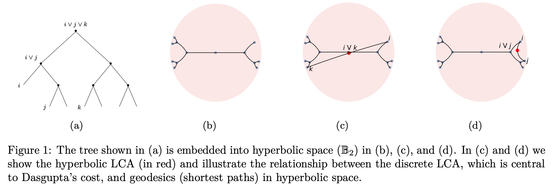
where \(i \lor j\) is the least common ancestor of \(i\) and \(j\). This is a very natural cost function over hierarchical clusterings.

Computation proceeds in two steps:

• Compute \(\vert \texttt{leaves} (T [a] ) \vert\) for every vertex \(a\). This takes linear time with a depth-first traversal.
• Compute the least common ancestor \(i \lor j\) for each edge.

I implemented this some time back for data analysis. Below, the idea is illustrated in code.

But several more optimizations are possible. The LCA is fastest computed using some pre-processing with a classic procedure: Tarjan’s offline LCA algorithm. This takes nearly-linear¹ amortized time. Using this and other innovations, a more efficient implementation of Dasgupta’s cost is the one in the excellent scikit-network module (other implementations also exist). It’s completely equivalent to my implementation above, but uses a more efficient data structure to compute the least common ancestor.

CODE

import itertools, scipy
from scipy import sparse, cluster
import numpy as np
import anndata, scanpy as sc

sc.settings.verbosity = 0
#adta = get_gtex_snrnaseq(file_path='../GTEx_8_snRNAseq_atlas.h5ad', mode='all', num_subsample=30000)
adta = sc.read('../GTEx_8_snRNAseq_atlas_30k.h5ad')

sc.pp.neighbors(adta)
sc.tl.umap(adta)



def dasgupta_cost_fn(weights, lkgtree_mat):
    """Compute Dasgupta's (linear) cost function over clusterings w.r.t. weights (nonnegative similarities) [1]_ .

    By default normalizes LCA-based pairwise similarities to have maximum value 1, 
    and normalizes weights to be a probability distribution over edges, so distance is in [0,1].

    Parameters
    ----------
    weights : sparse matrix
        Adjacency matrix of the input graph.
    lkgtree_mat : array
        Linkage matrix of the clustering.
    
    Returns
    -------
    dist : float
        Dasgupta's distance between the clusterings.
    
    References
    ----------
    .. [1] S. Dasgupta, A cost function for similarity-based hierarchical clustering, 
    Proceedings of the forty-eighth annual ACM symposium on Theory of Computing (pp. 118-127), 2016. 
    """
    # For each pair (i,j), compute (number of leaves - 1) subtended by the least common ancestor of (i,j).
    lcawts = scipy.sparse.csr_matrix(weights.shape)
    ttree = scipy.cluster.hierarchy.to_tree(lkgtree_mat, rd=True)
    data_clusters = {}
    for y in ttree[1]:
        if y.is_leaf():
            data_clusters[y.id] = [y.id]
            continue
        else:
            data_clusters[y.id] = data_clusters[y.left.id] + data_clusters[y.right.id]
    # Each split in the graph defines the LCA for the pairs of points cut by the split.
    for cl_id in data_clusters:
        if not ttree[1][cl_id].is_leaf():
            a1 = data_clusters[ttree[1][cl_id].left.id]
            a2 = data_clusters[ttree[1][cl_id].right.id]
            # Now connect all pairs of points with the lcawts, the weight of their LCA subtree.
            arr_ndces = list(zip(*list(itertools.product(a1, a2))))
            arr_ndces_rev = list(zip(*list(itertools.product(a2, a1))))
            lcawts[arr_ndces[0], arr_ndces[1]] = ttree[1][cl_id].count
            lcawts[arr_ndces_rev[0], arr_ndces_rev[1]] = ttree[1][cl_id].count
    # Normalize appropriately and return.
    lcawts = lcawts#*(1.0/ttree[0].count)
    wt_dist = weights/weights.sum()
    return lcawts.multiply(wt_dist).sum()

CODE

from sknetwork.data import karate_club
from sknetwork.hierarchy import Paris, cut_straight, dasgupta_cost, tree_sampling_divergence
from sknetwork.visualization import svg_graph, svg_bigraph, svg_dendrogram
from IPython.display import SVG

graph = karate_club(metadata=True)
adjacency = graph.adjacency
position = graph.position

# hierarchical clustering
paris = Paris()
dendrogram = paris.fit_predict(adjacency)

n_clusters = 4
labels, dendrogram_aggregate = cut_straight(dendrogram, n_clusters, return_dendrogram=True)
print(labels)


image = svg_dendrogram(dendrogram)
SVG(image)

[0 0 0 0 3 3 3 0 1 0 3 0 0 0 1 1 3 0 1 0 1 0 1 2 2 2 2 2 2 2 1 2 1 1]

CODE

# corresponding clustering
image = svg_graph(adjacency, position, labels=labels)
SVG(image)

CODE

dasgupta_cost(adjacency, dendrogram)

11.37179487179487

This cost function is a very natural one for multiple reasons, described beautifully in (Dasgupta 2016). It’s also related to the optimal transport distance between two distributions on an embedding induced by the tree (Le et al. 2019).

A KL divergence-based cost function

Another metric along these lines for the goodness of the hierarchy \(T\) is a clean information-theoretic one by (Charpentier and Bonald 2019). It’s based on the KL divergence between two distributions induced by the tree.

To describe these distributions, define \(u_i = \sum_{j} w_{i j}\). Then \(u\) and \(w\) induce two distributions over the nodes of the graph: \[ p (x) \propto \sum_{i \lor j = x} w_{i j} \qquad , \qquad q (x) \propto \sum_{i \lor j = x} u_i u_j \]

And the metric we’re interested in is the KL divergence between these two distributions over the tree \(\mathcal{T}\): \[ \text{TSD} (T) = \sum_{x \in T} p(x) \log \frac{p(x)}{q(x)} \]

This is higher if the tree faithfully matches the structure of the graph. As (Charpentier and Bonald 2019) write:

We expect these distributions to differ significantly if the tree indeed represents the hierarchical structure of the graph. Specifically, we expect p to be mostly concentrated on deep nodes of the tree (far from the root), as two nodes u, v connected with high weight w(u, v) in the graph typically belong to a small cluster, representative of the clustering structure of the graph; on the contrary, we expect q to be concentrated over shallow nodes (close to the root) as two nodes u, v sampled independently at random typically belong to large clusters, less representative of the clustering structure of the graph.

The canonical implementation of this, which is quite efficient on large graphs, is in the scikit-network module.

CODE

tree_sampling_divergence(adjacency, dendrogram)

0.3530310298063937

Hyperbolic spaces and trees

Hyperbolic geometry

The geometry of trees turns out to be very related to what are called negatively curved manifolds in mathematics. At any point on a manifold, negative curvature is the property of being curved “outwards” from the point, so that triangles appear pinched inwards.²

We can see that trees are “negatively curved” by looking at the triangles formed by three points on the tree. Distances between points become larger as we move away from the root, resulting in very “pinched” triangles.

The great geometer Gromov pioneered the study of hyperbolic spaces, leading to the Gromov product defined on a metric space \((X, d)\): \[ (y, z)_{x} := \frac{1}{2} \left( d(x, y) + d(x, z) - d(y, z) \right) \] which measures the closeness of \(x\) to the geodesic connecting \(y\) and \(z\). Hyperbolic spaces have \((y, z)_{x} - \min ( (y, w)_{x} , (z, w)_{x} ) \geq 0\) for all points \(w, x, y, z\), quantifying the intuition about triangles above. More discussion of hyperbolic spaces is at (Sala et al. 2018), which introduces a rigorously justified version of hyperbolic MDS.

Embedding in Euclidean space

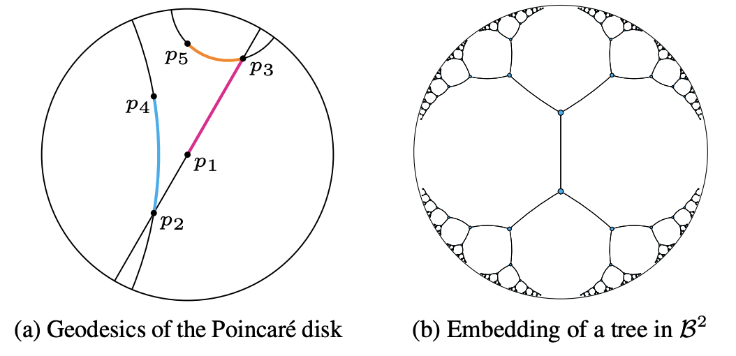
A nice way to embed a (non-Euclidean) hyperbolic space into Euclidean space is called the Poincaré ball (Maximilian Nickel and Kiela 2017), or disk in \(\mathbb{R}^2\).

As we see, this embeds hyperbolic space in a Euclidean ball, with geodesics being circular arcs that are perpendicular to the boundary. When trees are embedded in this space, they are rooted at the origin – the center of the ball – and the depth of any node is indicated by its distance from the origin.³

This embedding hugely simplifies LCA/subtree calculations, which are staples of hierarchical analysis, as we’ve been seeing.

• The LCA of two points is the closest point to the origin (the root) that is also on the geodesic connecting the two points.
• The subtree from a point \(x\) is a set such that the LCA of any two points in it is still in the set.

These are illustrated here, and can be calculated easily.

Though the Poincaré ball is most common and has appealing LCA geometry, there are other Euclidean embeddings of hyperbolic spaces. For instance, the Lorentz embedding notably has closed-form expressions for geodesics, and can perform empirically better in low dimensions (Maximillian Nickel and Kiela 2018).

Learning trees from metrics

The work of (Sonthalia and Gilbert 2020) introduces a way to learn a tree structure from pairwise affinities between data, which I like for the empirical simplicity and speed of its implementation, as well as the memorable title that inspired this post. The paper itself discusses the derivation of the method, which is based on a careful case analysis of possible tree structures in the fully recoverable case. A strong baseline for such tree construction/recovery methods is just using a minimum spanning tree over the pairwise affinity graph. This performs strongly even against state-of-the-art implementations to learn a tree structure on the data directly.

My personal favorite in this category is an algorithm that builds upon diffusion maps (discussed in another post) to learn in hyperbolic spaces (Lin et al. 2023). Unlike the others, this ends up learning an expanded representation of the data instead of compressing it. It learns a multi-scale embedding over the data, explicitly learning kernelized embeddings of the dataset at different scales by attentuating the lower- and higher-frequency components of the dataset. And it only requires one graph Laplacian eigenvalue decomposition.

There are a couple of adaptations to the original implementation that make it even faster. I may try those out in another post.

CODE

""" Adapted from the code of https://github.com/Ya-Wei0/HyperbolicDiffusionDistance .
"""


import numpy as np 
from sklearn.metrics import pairwise_distances


TOL = 1e-6


def hyperbolic_diffusion(ev, left_evv, right_evv, K):

    X_hat, hdd = [], [], []
    single_mat = []
    time_step = 1/np.power(2, np.arange(K))
    weight    = 2/np.power(2, np.arange(K)/2)

    for ii in range(len(time_step)):
        evv_power = np.power(ev, time_step[ii])

        x_hat = (left_evv @ np.diag(evv_power) @ right_evv)
        x_hat = np.sqrt(np.where(x_hat>TOL, x_hat, TOL))
   
        single_mat.append((2 * np.arcsinh( weight[ii] * pairwise_distances(x_hat))))
        
        tmp = np.concatenate((x_hat, (1/(2*weight[ii])) * np.ones((left_evv.shape[0], 1))), axis = 1)
        X_hat.append(tmp)

    hdd = np.sum(single_mat, axis = 0)
    
    return X_hat, hdd

The cluster tree

Clustering is a slippery problem to define, because the resolution of the structure to be detected is inconsistently or poorly defined. The intuitive way to define clusters when data are drawn from a density \(f\) is on the basis of level sets of \(f\): \[F_{\lambda} := \{x: f(x) \geq \lambda\} \] at a level \(\lambda\), which defines clusters as contiguous “islands” of density. Instead of fixing some arbitrary \(\lambda\), typically we simply sweep over \(\lambda\); as visible in the figure, decreasing \(\lambda\) causes the clusters to merge, mapping out a hierarchical cluster tree.

We do not know \(f\), and would like to estimate the cluster tree using samples from \(f\). The best-known approach for this task is simple in practice and comprehensive in theory (Chaudhuri and Dasgupta 2010). It is a robust version of a single linkage algorithm that greedily builds the cluster tree by merging the two closest clusters at each step.⁴ The package hdbscan specializes in efficient implementations of this type of “density-based” agglomerative clustering procedure, and we use it to estimate the cluster tree.

CODE

import hdbscan

def rsl_cluster_tree(data, knn_k=10):
    """Estimates the cluster tree by running robust single linkage, returning the resulting linkage matrix.
    """
    # cut is completely arbitrary because we're returning the whole tree anyway, so choose 0.5
    rsl_tree = hdbscan.RobustSingleLinkage(cut=0.5, k=knn_k)
    rsl_tree.fit(data.astype('float64'))
    return rsl_tree.cluster_hierarchy_.to_numpy()

Top-down clustering by recursive bipartitioning

Recursive (“top-down”) partitioning is a method used to partition a graph into clusters. Relative to agglomerative (“bottom-up”) clustering, it has the major advantage of no predefined resolution - it’s easy to adapt to situations where data arrive incrementally. This same characteristic leads to efficiency, interpretability, and robustness benefits as well.

Recursive spectral bipartitioning can be applied to hierarchically cluster a graph; it is a top-down approach that recursively divides the graph into two reasonably balanced parts, as in spectral clustering, until some stopping criteria are met.

This procedure has robust theory supporting it – the cost function of (Dasgupta 2016) is approximately minimized by its output ((Cohen-Addad et al. 2019) is a good reference on this active field).

Spectral bipartitioning

The core of this approach in practice is spectral graph bipartitioning, which leverages the eigenvectors of a graph’s Laplacian matrix to partition the graph into two parts. The eigenvector corresponding to the second smallest eigenvalue of the Laplacian (also known as the Fiedler vector) is used to divide the graph into two parts using the sign of the Fiedler vector components. This is a standard algorithm with many great tutorials.

Recursive bipartitioning

This spectral bipartitioning process is applied recursively to each of the subgraphs, partitioning them further and further until the desired number of clusters is reached or until some other stopping criteria are met.

Applying this process recursively builds up a hierarchy of clusters. At each level of the recursion, the clusters are divided further, resulting in a tree-like structure that represents the hierarchical clustering of the data.

CODE

from sklearn.cluster import SpectralClustering
import scipy

def spectral_bipartitioning(adj_mat):
    e = randomized_svd(adj_mat, n_components=2, n_iter=5, random_state=None)
    cluster_vals = e[0][:,1]
    cluster_lbls = np.array(cluster_vals > 0).astype(int)
    return cluster_lbls


def recursive_spectral_bipartitioning(adj_mat, max_depth=3, depth=0):
    """Recursively bipartitions the adjacency matrix using spectral clustering.
    """
    if depth >= max_depth:
        return np.zeros(adj_mat.shape[0])
    z = np.sqrt(np.asarray(adj_mat.sum(axis=0)).astype(np.float64))    # sqrt(density)
    recipsqrt = np.reciprocal(z)
    recipsqrt[np.isinf(recipsqrt)] = 0
    Zmat = scipy.sparse.spdiags(recipsqrt, 0, adj_mat.shape[0], adj_mat.shape[0])
    adj_mat = Zmat.dot(adj_mat).dot(Zmat)
    bipartition = spectral_bipartitioning(adj_mat)
    return bipartition
    clusters = np.zeros((max_depth - depth, bipartition.shape[0]))
    left_indices, right_indices = np.where(bipartition == 0)[0], np.where(bipartition == 1)[0]
    print(left_indices.shape, right_indices.shape, depth)
    subclusters_left = recursive_spectral_bipartitioning(adj_mat[np.ix_(left_indices, left_indices)], max_depth=max_depth, depth=depth+1)
    subclusters_right = recursive_spectral_bipartitioning(adj_mat[np.ix_(right_indices, right_indices)], max_depth=max_depth, depth=depth+1)
    print(subclusters_left.shape, clusters.shape, depth)
    clusters[:, left_indices] = subclusters_left
    clusters[:, right_indices] = subclusters_right
    clusters = np.vstack([bipartition, clusters])
    return clusters

adj_mat = a.obsp['connectivities']
mm = recursive_spectral_bipartitioning(adj_mat, max_depth=3)

References

Charpentier, Bertrand, and Thomas Bonald. 2019. “Tree Sampling Divergence: An Information-Theoretic Metric for Hierarchical Graph Clustering.” In Proceedings of the 28th International Joint Conference on Artificial Intelligence, 2067–73.

Chaudhuri, Kamalika, and Sanjoy Dasgupta. 2010. “Rates of Convergence for the Cluster Tree.” In Proceedings of the 23rd International Conference on Neural Information Processing Systems-Volume 1, 343–51.

Cohen-Addad, Vincent, Varun Kanade, Frederik Mallmann-Trenn, and Claire Mathieu. 2019. “Hierarchical Clustering: Objective Functions and Algorithms.” Journal of the ACM (JACM) 66 (4): 1–42.

Dasgupta, Sanjoy. 2016. “A Cost Function for Similarity-Based Hierarchical Clustering.” In Proceedings of the Forty-Eighth Annual ACM Symposium on Theory of Computing, 118–27.

Le, Tam, Makoto Yamada, Kenji Fukumizu, and Marco Cuturi. 2019. “Tree-Sliced Variants of Wasserstein Distances.” In Proceedings of the 33rd International Conference on Neural Information Processing Systems, 12304–15.

Lin, Ya-Wei Eileen, Ronald R Coifman, Gal Mishne, and Ronen Talmon. 2023. “Hyperbolic Diffusion Embedding and Distance for Hierarchical Representation Learning.” arXiv Preprint arXiv:2305.18962.

Nickel, Maximilian, and Douwe Kiela. 2017. “Poincaré Embeddings for Learning Hierarchical Representations.” In Proceedings of the 31st International Conference on Neural Information Processing Systems, 6341–50.

Nickel, Maximillian, and Douwe Kiela. 2018. “Learning Continuous Hierarchies in the Lorentz Model of Hyperbolic Geometry.” In International Conference on Machine Learning, 3779–88. PMLR.

Sala, Frederic, Chris De Sa, Albert Gu, and Christopher Ré. 2018. “Representation Tradeoffs for Hyperbolic Embeddings.” In International Conference on Machine Learning, 4460–69. PMLR.

Sonthalia, Rishi, and Anna Gilbert. 2020. “Tree! I Am No Tree! I Am a Low Dimensional Hyperbolic Embedding.” Advances in Neural Information Processing Systems 33: 845–56.

Footnotes

1. A rare use of the mathematically interesting inverse Ackermann function.

2. As opposed to the more familiar positive curvature of a sphere, where triangles appear pinched outwards.

3. Geodesics through the origin are diameters of the ball, and therefore straight lines.

4. The algorithm itself, roughly speaking, merges neighbors that are already in high-density regions.