Low-rank approximation of matrices and graphs

Efficient, robust, simple, and interpretable

Kernel matrices include graphs and other common types of distance-like matrices between data. They’re very common in exploratory data analysis to nonparametrically learn relationships (with very relaxed modeling assumptions) in datasets. In areas like genomics, it’s common for the kernel matrices to involve thousands or even millions of data points.

Such cases demand efficient algorithms for low-rank approximation of kernel matrices. There’s one in particular that will be explored here, because among other low-rank approximation methods, it’s:

• Efficient - requires just as much time/space as manipulating the reduced representation, not the data.
• Robust, simple, and interpretable

Approximating matrices: the Nyström method

The Nyström method is the prototype low-rank approximation method for kernel matrices. It efficiently finds a low-rank approximation of any kernel matrix, in a simple and interpretable way, using a subset of the matrix’s columns.

The method

Given a kernel matrix \(K \in \mathbb{R}^{n \times n}\), and a subset \(S\) of its columns, the Nyström method finds an approximation \(\hat{K}\) with rank \(k \ll n\).

Suppose we represent \(K\) as a block matrix, permuted so that the initial indices are \(S\):

\[ K = \begin{bmatrix} K_{SS} & K_{SU} \\ K_{US} & K_{UU} \end{bmatrix} \]

where \(K_{SS} \in \mathbb{R}^{k \times k}\), \(K_{SU} \in \mathbb{R}^{k \times (n-k)}\), and \(K_{US} \in \mathbb{R}^{(n-k) \times k}\). Then the Nyström approximation is:

\[ \hat{K} = \begin{bmatrix} K_{SS} \\ K_{US} \end{bmatrix} K_{SS}^{-1} \begin{bmatrix} K_{SS} & K_{SU} \end{bmatrix} \]

Extensions

More generally, the “Nyström approximation” can be defined even without using a subset of rows, instead using a more general \(n \times k\) “test matrix” \(X\) to probe \(A\). When \(A X\) selects the desired subset of columns of \(A\), this is equivalent to the idea explained above.

In this post, we’ve seen that a column Nyström approximation can be obtained from a partial Cholesky decomposition. The residual of the approximation is the Schur complement - as (Martinsson and Tropp 2020) states, “the Schur complement of A with respect to X is precisely the error in the Nystrom¨ approximation.”

Schur complement and Cholesky factorization

The Cholesky factorization of \(A\) basically logs the results of using the Gaussian elimination algorithm to solve a system of linear equations parametrized by \(A\). It decomposes \(A\) into a product of a lower triangular matrix \(L\) and its transpose \(L^T\), and the sparsity pattern is often highly interpretable in practice.

The Schur complement of \(A\) with respect to a subset of its rows is exactly the difference between \(A\) and its Nyström approximation using those rows. It describes what remains after eliminating the corresponding constraints from \(A\). These are intimately related in theory and practice – here’s a nice summary.

Computing the approximate matrix

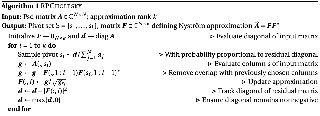
A massive field of literature surveys how to solve this low-rank Nyström approximation problem, with methods based on ridge leverage score sampling being a particular highlight. But recently, a simple algorithm has emerged that is very efficient and gives exactly what is needed (we refer to the version from (Chen et al. 2022)).

Figure 1: The Nyström approximation algorithm.

This can be implemented as follows.

import numpy as np

def low_rank_cholesky(A, n_rank):
    """ Computes a low rank Cholesky decomposition of A. 

    Parameters
    ----------
    A : ndarray
        The matrix to decompose.
    n_rank : int
        The rank of the decomposition.
    
    Returns
    -------
    F : ndarray
        The lower triangular matrix of the decomposition.
    arr_idx : ndarray
        The indices of the selected elements used in the decomposition.

    Notes
    -----
    Adapted from the source at https://github.com/eepperly/Randomly-Pivoted-Cholesky .
    """
    n = A.shape[0]
    diags = A.diag()
    
    # row ordering, is much faster for large scale problems
    F = np.zeros((n_rank,n))
    rng = np.random.default_rng()
    arr_idx = []
    for i in range(n_rank):
        idx = rng.choice(range(n)
        p = diags / np.sum(diags))
        F[i,:] = (A[idx,:] - F[:i,idx].T @ F[:i,:]) / np.sqrt(diags[idx])
        diags -= F[i,:]**2
        diags = diags.clip(min = 0)
        arr_idx.append(idx)
    return F.T, arr_idx

Usage

The Nyström approximation is a very useful tool for exploratory data analysis in “compressing” a symmetric PSD matrix of data, like a kernel matrix or a covariance matrix.

Typically, a random sample of the data is taken, and the Nyström approximation is computed using that sample. This is bottlenecked by the complexity of taking a matrix inverse, or a Cholesky decomposition, which is \(O(k^3)\) for a \(k \times k\) matrix.

The algorithm we have here has a couple of important differences from that approach:

• It adaptively selects the sample \(S\) with randomness, but in a structured way. This subset is itself quite interesting, as an actively selected set of the most representative landmark points in the Nyström sampling.
• It decomposes \(A\), returning the Cholesky decomposition \(A \approx F F^{\top}\) as a byproduct, with lower-triangular \(F\) expressing the low-rank factors as interpretable mixtures of \(A\)’s columns.

References

Chen, Yifan, Ethan N Epperly, Joel A Tropp, and Robert J Webber. 2022. “Randomly Pivoted Cholesky: Practical Approximation of a Kernel Matrix with Few Entry Evaluations.” arXiv Preprint arXiv:2207.06503.

Martinsson, Per-Gunnar, and Joel A Tropp. 2020. “Randomized Numerical Linear Algebra: Foundations and Algorithms.” Acta Numerica 29: 403–572.