Solving sparse linear equations

Logging the results of Gaussian elimination

Solving sparse systems of linear equations

Sparse linear systems $ A = $ arise in countless applications, from scientific simulations to machine learning. When the matrix \(A\) is large and mostly zeros (sparse), such as for graph-based learning, specialized techniques are needed to solve for \(\mathbf{x}\) efficiently.

There are two broad classes of solvers: direct methods that perform matrix factorizations (like Gaussian elimination), and iterative methods that progressively refine an approximate solution. All these methods are workhorses of modern numerical implementations, and are so important in practical settings that they bear further mention. They are useful not only in situations where there is a well-defined solution to the equations, but also in the underdetermined and overdetermined settings that characterize practical data science, where the equations themselves are defined by data or models.

One iterative method stands out: the conjugate gradient (CG) method is considered one of the great algorithms of the 20th century. It is simple and efficient, and its analysis is a beautiful illustration of several concepts in numerical linear algebra. In practical terms, CG is often the method of choice for large-scale problems where direct solvers (like Gaussian elimination or Cholesky factorization) become infeasible due to time or memory.

In addition to diving into CG, we will compare and contrast it with direct methods such as sparse Cholesky factorization, since these provide important baselines and are also staple tools of linear algebra with sparse matrices. All these algorithms come from a basic toolkit of randomized linear algebra methods, which have largely only been developed in the past decade or two and enable massive speedups. Therefore, the algorithms typically implemented for these purposes in the 2020s are quite different than the ones used even in 2010.

Connecting Schur complements, Cholesky factorizations, and linear systems

Since we are talking about matrices \(A\), everything can be stated in the language of linear systems \(A x = b\). It is most convenient to view all these methods as different perspectives on the fundamental method of Gaussian elimination applied to solve linear systems.

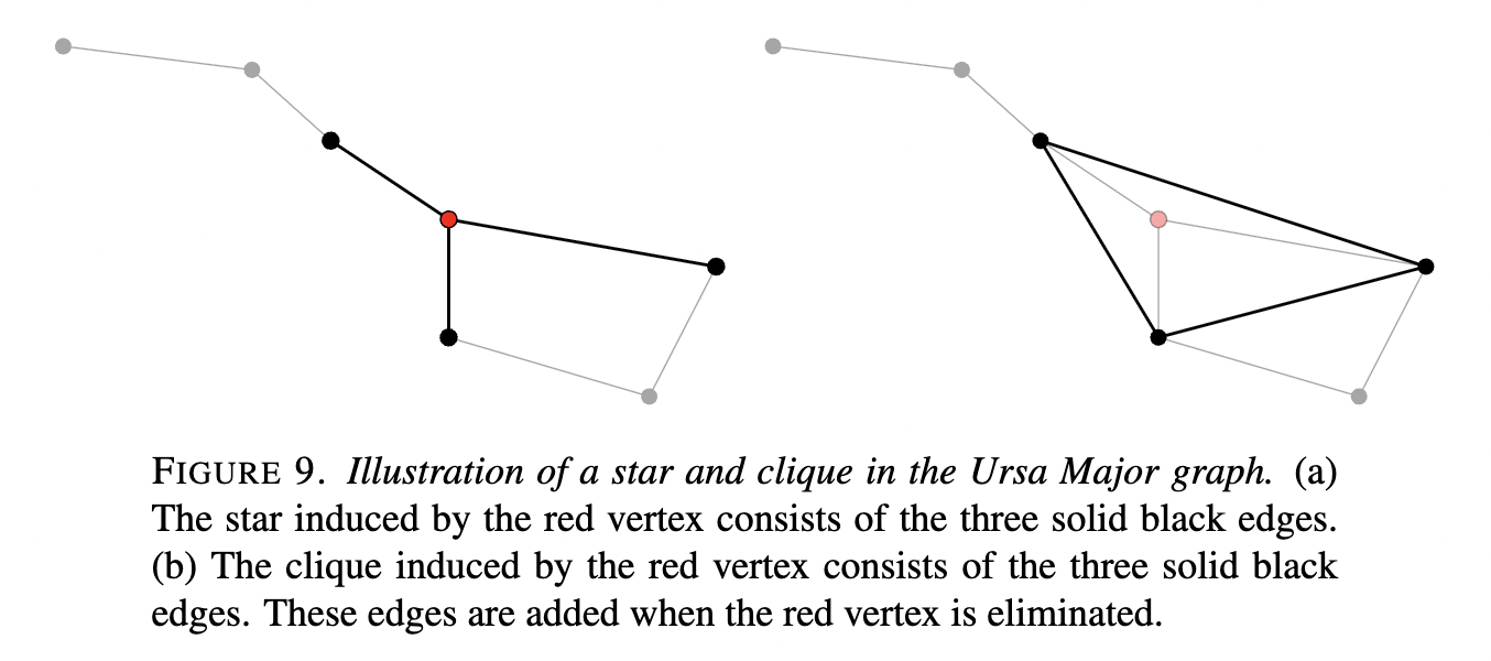
Schur complements represent reduced linear systems – the objects that arise when part of the system is eliminated (e.g. in Gaussian elimination). They preserve SPD-ness when \(A\) is SPD. Therefore, the Schur complement of any graph with respect to all the nodes except a node \(v_1\) (which gets eliminated) is obtained by removing the \(\text{STAR}\) graph induced by \(v_1\) and add the \(\text{CLIQUE}\) graph induced by \(v_1\) (Kothapalli 2023). These are illustrated in (Martinsson and Tropp 2020):

Figure 1: Figure 9 in (Martinsson and Tropp 2020).

Schur complements also have various properties that connect them intimately to effective resistances on graphs and random walks. The details are a subject of active interest, and enable state-of-the-art methods (See (Gao, Liu, and Peng 2023), Sec. 4.1).

As we’ve seen, Cholesky factorizations essentially log the process of Gaussian elimination, and when a variable is eliminated, the updated Cholesky factor is now of the new Schur complement matrix. For any SPD A with Cholesky decomposition \(A = L L^{\top}\), \[ A = \begin{bmatrix} a_{11} & a_{12}^{\top} \\ a_{12} & A_{22} \end{bmatrix} \qquad \to \qquad L = \begin{bmatrix} \sqrt{a_{11}} & 0 \\ \frac{a_{12}}{\sqrt{a_{11}}} & L_{22} \end{bmatrix} \] where \(L_{22}\) is the Cholesky factor of the Schur complement \[ S = A_{22} - \frac{1}{a_{11}} a_{12} a_{12}^{\top} \]

So a Cholesky decomposition is a systematic way of doing elimination for SPD systems, repeatedly forming Schur complements, until the whole factorization is built.

To summarize,

• Linear system: We want to solve \(Ax=b\).

• Schur complements: Appear when eliminating part of the system (block Gaussian elimination).

• Cholesky factorization: A systematic way of doing elimination for SPD systems, repeatedly forming Schur complements, until the whole factorization is built.

Conjugate gradient iteration

Developed by Hestenes and Stiefel in 1952 (Hestenes, Stiefel, et al. 1952), CG is today the standard algorithm for solving very large sparse systems that are symmetric and positive-definite. The basic idea is to avoid the costly matrix factorizations required by direct methods by instead iteratively refining an approximate solution. At each step, CG chooses a smart search direction that is “conjugate” (perpendicular in an \(A\)-inner-product sense) to previous search directions, ensuring that progress made in one direction is not lost in subsequent steps. By doing so, it converges to the exact solution in at most \(n\) steps in exact arithmetic (for an \(n\times n\) system), although in practice far fewer iterations are needed for a good approximation. In all its forms, the conjugate gradient method is the most prominent iterative method for solving sparse linear systems, combining the reliability of direct solvers with the low per-iteration cost of simple iterative schemes.

The conjugate gradient algorithm solves a linear system \(A\mathbf{x} = \mathbf{b}\) by minimizing the quadratic error function \(f(\mathbf{x}) = \frac{1}{2}\mathbf{x}^{\top} A \mathbf{x} - \mathbf{x}^{\top} \mathbf{b}\) (which is convex when \(A\) is symmetric positive-definite). At each iteration, CG chooses a search direction that is conjugate (or \(A\)-orthogonal) to all previous search directions, ensuring that progress made in one direction is not undone by later steps. This is an improvement over the basic steepest descent (gradient descent) method, which always moves in the direction of the residual (the negative gradient) and often “zig-zags” inefficiently between directions.

Comparison with steepest descent

Steepest descent recap: Starting from an initial guess \(\mathbf{x}_0\), the residual is \(\mathbf{r}_0 = \mathbf{b} - A\mathbf{x}_0\). Steepest descent would set \(\mathbf{p}_0 = \mathbf{r}_0\) and update \(\mathbf{x}_{1} = \mathbf{x}_0 + \alpha_0 \mathbf{p}_0\) with step size \(\alpha_0 = \frac{\mathbf{r}_0^{\top} \mathbf{r}_0}{\mathbf{p}_0^{\top} A \mathbf{p}_0}\) chosen to minimize \(f(\mathbf{x})\) along \(\mathbf{p}_0\). Then the process repeats: \(\mathbf{p}_1 = \mathbf{r}_1 = \mathbf{b} - A\mathbf{x}_1\), etc. Steepest descent converges on these problems, but can be extremely slow when \(A\) has a large condition number (eigenvalues spread apart), because the error reduction per iteration is bounded by a factor \(\frac{\kappa-1}{\kappa+1}\) (where \(\kappa\) is \(A\)’s condition number) in the best case.

Conjugacy and optimal directions: The key idea of CG is to construct search directions \(\mathbf{p}_0, \mathbf{p}_1, \dots\) that are mutually conjugate with respect to \(A\) (i.e. \(\mathbf{p}_i^{\top} A \mathbf{p}_j = 0\) for \(i\neq j\)). Intuitively, this means each new direction is chosen to eliminate error components that were not addressed by previous steps. In fact, CG can be viewed as the method of conjugate directions, but where each new direction is obtained conveniently by adjusting the latest residual. At iteration \(k\), after \(k\) conjugate directions, CG has minimized the error over the \(k\)-dimensional “Krylov subspace” \(\mathcal{K}_k = \mathrm{span}\{\mathbf{r}_0, A\mathbf{r}_0, \,A^2\mathbf{r}_0, \dots, A^{k-1}\mathbf{r}_0\}\), and the error \(\mathbf{e}_k = \mathbf{x}_k - \mathbf{x}_*\) (difference from the true solution) is orthogonal to this subspace. Consequently, in exact arithmetic CG converges in at most \(n\) iterations, and often much sooner if the eigenvalues of \(A\) cluster.

Algorithm outline

Starting from an initial guess \(\mathbf{x}_0\) (often the zero vector), CG works as follows. We maintain an iterate \(\mathbf{x}_k\), a residual \(\mathbf{r}_k = \mathbf{b} - A\mathbf{x}_k\) (which is the negative gradient of \(f\) at \(\mathbf{x}_k\)), and a search direction \(\mathbf{p}_k\).

We initialize \(\mathbf{x}_0\) (e.g. the zero vector) and \(\mathbf{r}_0 = \mathbf{b} - A\mathbf{x}_0\), \(\mathbf{p}_0 = \mathbf{r}_0\). Then for each iteration \(k=0,1,2,\ldots\):

1. Compute the optimal step length along \(\mathbf{p}_k\) that minimizes \(f(\mathbf{x}_k + α \mathbf{p}_k)\): \[ \alpha_k = \frac{\mathbf{r}_k^{\top} \mathbf{r}_k}{\mathbf{p}_k^{\top} A \mathbf{p}_k} \]
2. \(\mathbf{x}_{k+1} = \mathbf{x}_k + \alpha_k \mathbf{p}_k\) (update solution)
3. \(\mathbf{r}_{k+1} = \mathbf{r}_k - \alpha_k A \mathbf{p}_k\) (compute new residual)
4. If \(\|\mathbf{r}_{k+1}\|\) is below tolerance, break (converged)
5. Compute conjugate direction coefficient \[ \beta_k = \frac{\mathbf{r}_{k+1}^{\top} \mathbf{r}_{k+1}}{\mathbf{r}_k^{\top} \mathbf{r}_k} \]
6. \(\mathbf{p}_{k+1} = \mathbf{r}_{k+1} + \beta_k \mathbf{p}_k\) (new search direction, \(A\)-conjugate to previous)

This procedure is remarkably simple computationally (only a few vector operations and one \(A\)-matrix-vector product per iteration). Yet it guarantees optimal error reduction in the \(k\)-dimensional search subspace at each step (Shewchuk 1994). Below we compare the convergence of steepest descent and conjugate gradient on a small example problem.

import numpy as np
# (Set up A, b, x0 and define steepest_descent and conjugate_gradient as above)
# ... [see source code for full implementation] ...
n = 50
cond_num = 100.0
Q, _ = np.linalg.qr(np.random.randn(n, n))
eigs = np.linspace(1, cond_num, n)
A = Q.T @ np.diag(eigs) @ Q
x_true = np.ones(n); b = A.dot(x_true); x0 = np.zeros(n)


def steepest_descent(A, b, x0, maxiters=50):
    x = x0.copy()
    r = b - A.dot(x)
    res_norms = [np.linalg.norm(r)]
    for k in range(maxiters):
        Ar = A.dot(r)
        alpha = r.dot(r) / r.dot(Ar)
        x = x + alpha * r
        r = r - alpha * Ar
        res_norms.append(np.linalg.norm(r))
    return res_norms

def conjugate_gradient(A, b, x0, maxiters=50):
    x = x0.copy()
    r = b - A.dot(x); p = r.copy()
    res_norms = [np.linalg.norm(r)]; rr = r.dot(r)
    for k in range(maxiters):
        Ap = A.dot(p)
        alpha = rr / p.dot(Ap)
        x = x + alpha * p
        r = r - alpha * Ap
        new_rr = r.dot(r)
        res_norms.append(np.linalg.norm(r))
        if np.sqrt(new_rr) < 1e-12:
            break
        beta = new_rr / rr
        p = r + beta * p
        rr = new_rr
    return res_norms


res_sd = steepest_descent(A, b, x0, maxiters=50)
res_cg = conjugate_gradient(A, b, x0, maxiters=50)


print(f"Residual after 50 iterations (Steepest Descent): {res_sd[-1]:.2e}")
print(f"Residual after 50 iterations (Conjugate Gradient): {res_cg[-1]:.2e}")

Residual after 50 iterations (Steepest Descent): 6.91e-01
Residual after 50 iterations (Conjugate Gradient): 5.90e-13

From the plot, we see that conjugate gradient rapidly reduces the residual by orders of magnitude, whereas steepest descent stagnates. In this example (matrix of size 50 with condition number 100), CG reached machine precision in about 15 iterations, whereas steepest descent made very slow progress.

The residual \(\mathbf{r}_k\) is always kept orthogonal to all previous search directions, and one can show that \(\mathbf{x}_k\) is the best possible approximate solution in the \(k\)-dimensional Krylov subspace \[ \mathcal{K}_k = \operatorname{span} \left( \mathbf{r}_0, A\mathbf{r}_0, \ldots, A^{k-1}\mathbf{r}_0 \right) \] This optimality perspective is another way to see why CG converges in \(n\) steps: \(\mathcal{K}_n = \mathbb{R}^n\), so the solution \(\mathbf{x}*\) lies in that subspace.

Theory

The theoretical convergence bound for CG confirms this efficiency. It’s written in terms of the induced matrix norm \(\| x \|_{A} := \sqrt{x^{\top} A x}\), which is the “right” way to measure error for the CG method in this situation. In fact, \(\| x \|_{A}\) can be broken into a sum, “each term [of which] is associated with a search direction that has not yet been traversed” (Shewchuk 1994).

After \(k\) iterations, \[ \frac{\|\mathbf{e}_k\|_A}{\|\mathbf{e}_0\|_A} \le 2\left(\frac{\sqrt{\kappa}-1}{\sqrt{\kappa}+1}\right)^k \]

which is roughly \(\left(1 - \frac{2}{\sqrt{\kappa}}\right)^k\) for large \(\kappa\).

In contrast, basic iterative methods like Jacobi or Gauss-Seidel have error factors on the order of \(2\left(\frac{\kappa - 1}{\kappa + 1}\right)^k \approx 1 - 2/\kappa\) per iteration. The convergence rates of CG replace \(\kappa\) here by \(\sqrt{kappa}\), meaning CG can converge much faster for ill-conditioned problems.

Practical aspects

In practice, CG is typically used with a preconditioner \(M\) that approximates \(A^{-1}\) to improve convergence. Preconditioning effectively reduces the condition number of \(M^{-1}A\), leading to fewer iterations. A staple modern preconditioning method for large amounts of data computes a quick randomized Nyström approximation of the principal subspaces, to compress the eigenvalues into a smaller range and improve the stability of convergence (Martinsson and Tropp 2020).

In machine learning applications, it is common to stop CG after a limited number of iterations (or once the residual is “good enough”) rather than insist on a tiny residual – this trades off accuracy for time. Often just a few iterations of CG yield a large improvement (because the initial error components along high-eigenvalue directions are quickly eliminated), and diminishing returns set in for later iterations. This is one reason that sophisticated preconditioners may not always be worth it for ML tasks if moderate accuracy is acceptable. In summary, CG’s performance depends on the spectrum of \(A\); clustering of eigenvalues or a good preconditioner can lead to superlinear convergence in practice, whereas very ill-conditioned problems may still be slow (or require preconditioning to be tractable).

CG’s cost grows roughly linearly with \(N\) (each iteration is \(O(N)\) and required iterations grow sublinearly for many problems), whereas direct factorization cost grows superlinearly. In practice, beyond a certain problem size, iterative methods overtake direct methods in efficiency. Moreover, memory can become a bottleneck for direct solvers: factorizing a large sparse matrix can consume much more memory than storing the matrix itself, due to fill-in. CG avoids that by working with the matrix as a linear operator.

CG is implemented in libraries such as SciPy (see scipy.sparse.linalg.cg) and is a workhorse for large-scale problems in scientific computing and machine learning. For example, one can solve a least-squares problem \(\min_x \|Xw - y\|^2\) by applying CG to the normal equations \(X^{\top} X w = X^{\top} y\) instead of explicitly forming \(X^{\top} X\). However, forming the normal equations squares the condition number, so often it is better to use CG on \(X X^{\top}\) (CG on the normal equations is known as CGNR) or to use a preconditioner.

Sparse Cholesky factorization and graph structures

Before the conjugate gradient era, the standard way to solve \(A\mathbf{x}=\mathbf{b}\) was to factorize \(A\) directly using Gaussian elimination. For symmetric positive-definite matrices, the classic approach is Cholesky factorization, which computes a lower-triangular \(L\) such that \(A = LL^{\top}\). Solving then involves two triangular solves (\(L\mathbf{y} = \mathbf{b}\), then \(L^{\top} \mathbf{x} = \mathbf{y}\)) – forward- and back-substitution in two quick passes.

Cholesky is efficient for moderate-sized dense matrices, but for large sparse \(A\), the challenge is fill-in: \(L\) may have many more nonzero entries than \(A\). This fill-in depends on the matrix’s graph structure. In graph terms, eliminating a variable (corresponding to a row/column) connects all its neighbors together (forming a clique). If the graph of \(A\) is a chain or tree, no large cliques form and Cholesky stays sparse; but a more connected graph (e.g. a 2D grid or a social network) can lead to large cliques and heavy fill-in.

Strategies like reordering the matrix (finding an elimination order that minimizes clique sizes) are crucial in sparse direct solvers for CPU/GPU. For example, minimum-degree or “nested dissection” orderings can greatly reduce fill¹. Even so, some problems are so large that storing the factors \(L\) is impractical, much more than storing a sparse \(A\). This is where iterative solvers like CG shine: they access \(A\) only via matrix-vector products and don’t need to store additional large matrices.

On the other hand, if we need to solve many linear systems with the same \(A\) (multiple \(\mathbf{b}\)’s), computing a Cholesky factorization once and reusing it for fast solves can be advantageous. There is ongoing research into intermediate approaches, such as approximate factorizations. One example is the Randomized Cholesky algorithm, which uses random sampling to build an approximate \(L\) for graph Laplacians. Such techniques serve as powerful preconditioners for CG or enable faster direct solves by sacrificing some accuracy for speed.

Comparison with conjugate gradient

Conjugate gradient and sparse Cholesky represent two ends of a spectrum. CG is iterative, often memory-light, and benefits from lower precision requirements; Cholesky is direct, memory-heavy, but can solve in a fixed number of operations. In modern large-scale machine learning and scientific computing, CG and its extensions (like Lanczos-based methods and preconditioned variants) are indispensable for handling huge sparse systems, while sparse Cholesky and related direct methods remain vital for problems where factorization is feasible or multiple solves are needed.

Fill-in and graph interpretation

An intuitive way to understand fill-in is via graph theory. We can associate \(A\) with an undirected graph where each row/column variable is a node and each nonzero \(a_{ij}\) is an edge. Gaussian elimination (or Cholesky) corresponds to eliminating nodes from this graph. When a node is eliminated, all its neighbors become mutually connected (forming a clique) in the remaining graph. This clique represents the new fill-in edges. In other words, eliminating a variable “connects” every pair of variables that used to only be connected through that eliminated variable. If the graph of \(A\) is very connected or if our elimination order is unlucky, large cliques (complete subgraphs) can form and the factor \(L\) becomes dense in blocks. This is because of the connection between Gaussian elimination and Schur complements that we mentioned above: eliminating a vertex (forming a “star”) introduces a clique among its neighbors.

Sparse Cholesky algorithms therefore carefully choose the next node to eliminate (e.g. a minimum-degree node) to limit clique size and hence fill-in. Even so, some problems are so large (or graphs so dense) that factoring them is impractical, and CG is a boon for such situations.

Sparse direct vs. iterative

If we can afford it, direct factorization is extremely powerful. It is a one-time cost after which we can solve \(A \mathbf{x} = \mathbf{b}\) for multiple right-hand sides very cheaply. Direct methods are also robust and not sensitive to conditioning in the way iterative methods are (ill-conditioned systems will slow down CG, but Cholesky will still produce a solution in predictable time, barring numerical breakdown). In machine learning, a classic example is computing the solution to normal equations in linear regression or least squares: if \(X\) is a data matrix, solving \((X^{\top}X + λI) \mathbf{w} = X^{\top} \mathbf{y}\) via Cholesky (possibly with \(λI\) ridge regularization) will give the model weights in one shot.

For moderately sized datasets this is fine, but for very large ones, \(X^{\top} X\) becomes huge to factor. We instead rely on iterative solvers (CG or variants of stochastic gradient descent) to approximate the solution.

When \(n\) is in the millions (as can happen with big graph Laplacians or kernel matrices in ML), iterative solvers are often the only viable option. Even state-of-the-art sparse direct solvers can struggle due to memory limits: for instance, factoring a million-by-million sparse matrix might generate billions of nonzeros in \(L\) in the worst case. Iterative methods like CG, by contrast, do not need to explicitly form fill-in – they only interact with \(A\) via multiplications. This is why CG is “the most popular iterative method for solving large systems.” It’s important to note, though, that iterative methods yield a solution up to tolerance. If extremely high accuracy is needed or if the matrix is near-singular, a direct method (or extra precautions like higher precision arithmetic) might be necessary.

Enhancements

A lot of research has gone into bridging the gap between direct and iterative methods. One approach is incomplete factorization, where one computes a sparse approximation of \(L\) by dropping smaller fill-in entries – this can serve as an effective preconditioner for CG (e.g. ILU or IC preconditioners). Another exciting development in recent years is the use of randomized algorithms to accelerate linear solves. For example, randomized sparse Cholesky techniques sample the fill-in clique edges, retaining only a subset with probabilistic guarantees.

This can yield an approximate factor \(L\) that is much sparser (and faster to compute), at the cost of some accuracy. Such methods, combined with iterative refinement, have been applied to graph Laplacian systems – a notable result is that graph Laplacians can be solved in nearly-linear time with high probability using random projection and multilevel preconditioning (e.g. breakthroughs on “ultrasparsifiers”). In ML, related ideas include using Nyström approximations for kernel matrices (which is akin to randomly selecting rows/columns to approximate a factorization).

In a nutshell, sparse Cholesky factorization provides a powerful but memory-intensive baseline for solving \(A\mathbf{x}=\mathbf{b}\). Conjugate gradient and its family of Krylov subspace methods offer a complementary approach that trades exactness for scalability. In modern large-scale machine learning tasks, one often uses iterative methods – possibly preconditioned – to handle gigantic linear systems that would be impossible to factorize.
However, whenever the problem size permits or multiple solves are required, a sparse direct solve (or a hybrid strategy) can be the optimal choice.

The conjugate gradient method, together with related methods for preconditioners, Lanczos eigenanalysis, and other Krylov methods, form an indispensable toolkit for machine learning practitioners tackling large linear algebra problems. These methods are crucial to efficiently solve the sparse linear equations that arise throughout practical modern machine learning on large scientific data (Murray et al. 2023).

References

Gao, Yu, Yang Liu, and Richard Peng. 2023. “Fully Dynamic Electrical Flows: Sparse Maxflow Faster Than Goldberg–Rao.” SIAM Journal on Computing, no. 0: FOCS21–85.

Hestenes, Magnus R, Eduard Stiefel, et al. 1952. “Methods of Conjugate Gradients for Solving Linear Systems.” Journal of Research of the National Bureau of Standards 49 (6): 409–36.

Kothapalli, Vignesh. 2023. “Randomized Schur Complement Views for Graph Contrastive Learning.” In International Conference on Machine Learning, 17580–614. PMLR.

Martinsson, Per-Gunnar, and Joel A Tropp. 2020. “Randomized Numerical Linear Algebra: Foundations and Algorithms.” Acta Numerica 29: 403–572.

Murray, Riley, James Demmel, Michael W Mahoney, N Benjamin Erichson, Maksim Melnichenko, Osman Asif Malik, Laura Grigori, et al. 2023. “Randomized Numerical Linear Algebra: A Perspective on the Field with an Eye to Software.” arXiv Preprint arXiv:2302.11474.

Shewchuk, Jonathan Richard. 1994. “An Introduction to the Conjugate Gradient Method Without the Agonizing Pain.”

Footnotes

1. The effects can be dramatic: for example, an \(N\)-node 3D grid Laplacian can be factored in about \(O(N^{2})\) operations rather than \(O(N^{3})\).