Which data in a dataset are easier and harder to classify?
This is a basic question that people routinely want to answer about their data. The answer depends on the featurization and model.
When the data are approximately linearly separable, this question is answered in a satisfying and intuitive way by the margin of each point – its distance to the decision boundary. But in modern classification, the state of the art typically relies on a deep pipeline for embedding the data, and not on specific parameters that can be used to define a margin.
A paper of ours (Balsubramani et al. 2019) gives a nonparametric margin for each point – a way to view the difficulty of classifying any data point in an embedding – with principled and interpretable underpinnings. The algorithms and results remain exciting and fundamental when applying embeddings for industrial uses, and so this post explains them outside the academic setting.
Very commonly, we get an embedding in which some data are expressed. When we evaluate this embedding with respect to the label that was used to supervise it, linear classifiers often perform quite well – the embedding is learned such that the final-layer predictor, a linear classifier, performs well. But embeddings, particularly foundation models, are increasingly trained on multiple sources of input, and so the decision boundary in practice is often quite complex.
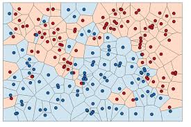
Voronoi diagram of k-NN regions
In this situation, it’s useful to have principled black-box ways of assessing uncertainty of a labeling on an embedding. Given an embedding and a little labeled data from it, where are the regions of high and low label uncertainty?
Why nearest neighbor
The labeling could be quite complicated, so we normally can’t assume very much about it. The “Bayes optimal classifier” is the best we can possibly do – it picks the label that we would pick if we completely knew the label distribution of the data. Even this can make mistakes, because of label noise that is outside the purview of what can be learned from this dataset. But we would like to use it to assess the embedding, because it represents the label function at all scales (coarse and fine).
Without knowing the Bayes optimal classifier, we want to assess what can be learned in light of existing labels. As we do not want to fall short of Bayes optimal, we can only use existing labels in a way that actually converges to the Bayes optimal classifier, given enough labels. Such methods are called “consistent”.
(Weighted) nearest-neighbor classifiers are the only consistent predictors over embeddings in practice.
This section is devoted to describing why.
It’s long been known that to get close to the best possible classification error, it makes sense to consider local neighborhood-based prediction rules that just take a few nearest neighbors ((Stone 1977), Stone 1980, Stone 1982). In fact, there are really no other such predictors that we need to consider in practice:
The rules we get should not change under rotations, translations, and other isometries (distance-preserving transformations). Also, the raw distances in the embedding offer some information, but it can be very brittle to learning dynamics; we’d want a prediction rule to stay unchanged under monotone distance transforms. Putting together standard group‑invariance reduction (Wijsman 1990) and ordinalinvariance ((Sidak, Sen, and Hajek 1999), (Eaton 1989)), any rule that honors isometries and monotone distance transforms can depend only on distance ranks.
Imposing locality (a finite neighborhood, i.e. finitely many neighbors influence the decision) restricts attention to the labels of the nearest \(k\) neighbors.
Under 0–1 (resp. squared) loss, the Bayes action is a majority vote (resp. average) over these labels, i.e., a nearest‑neighbor rule.
Combining these arguments, we see that under any loss, nearest neighbor rules are the ones that matter on any embedding. And when a particular loss function is clear (as often for 0-1 and squared losses above), its Bayes optimal prediction should be considered.
Nearest-neighbor classification
Among the oldest and best-known algorithms for classification is the \(k\)-nearest neighbor algorithm:
Classify each test point according to the labels of its \(k\)-neighborhood (\(k\) nearest neighbors) in the training set.
This is the prototype nonparametric classification method. It relies on the basic homophily assumption of nonparametric prediction methods – that “nearby” points have similar labels. Here is an implementation for illustration and use.
CODE
import numpy as np, scipy, time, scipy.io, sklearnimport sklearn.metricsfrom sklearn.neighbors import NearestNeighborsdef calc_nbrs_exact(raw_data, k=1000, query_is_ref=True): distances, indices = NearestNeighbors(n_neighbors=k+1).fit(raw_data).kneighbors(raw_data)return indices[:, 1:] if query_is_ref else indicesdef knn_rule(nbr_list_sorted, labels, k=10):""" For benchmarking: given matrix of ordered nearest neighbors for each point, returns kNN rule's label predictions. Parameters ---------- nbr_list_sorted: array of shape (n_samples, n_neighbors) Indices of the `n_neighbors` nearest neighbors in the dataset, for each data point. Returns ------- array of shape (n_samples) Predictions of the k-NN rule for each data point. """ toret = []for i inrange(nbr_list_sorted.shape[0]): uq = np.unique(labels[nbr_list_sorted[i,:k]], return_counts=True) toret.append(uq[0][np.argmax(uq[1])])return np.array(toret)
This is a toy implementation, for illustration more than for practical use at scale. There are a couple of reasons for this:
The neighbor-finding routine is almost always an approximate nearest neighbor (ANN) method. The exact neighborhood computation done here is much more cumbersome computationally, and quickly fails to scale compared to ANN (Aumüller, Bernhardsson, and Faithfull 2020).
The \(k\)-NN rule is implemented in scikit-learn and many other standard packages, so there is no reason to write this from scratch.
We build from the basics of this implementation to code the new algorithm.
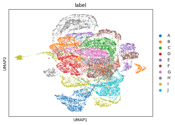
In this post, we follow the paper in illustrating these neighborhood-based algorithms on the notMNIST dataset, a more challenging version of the 10-class MNIST classification dataset. We demonstrate and document an entire package’s worth of functions that use the neighborhood graph for this task. First, we calculate and plot the landscape of labels on notMNIST.
CODE
# First download the dataset from http://yaroslavvb.com/upload/notMNIST/notMNIST_small.matimport urllib.requestimport osurl ="http://yaroslavvb.com/upload/notMNIST/notMNIST_small.mat"filename ="../../files/datasets/notMNIST_small.mat"ifnot os.path.exists(filename):print(f"Downloading {filename} from {url} ...") urllib.request.urlretrieve(url, filename)print("Download complete.")else:print(f"{filename} already exists. Skipping download.")
/opt/anaconda3/envs/env-dash/lib/python3.10/site-packages/anndata/_core/anndata.py:381: FutureWarning: The dtype argument is deprecated and will be removed in late 2024.
  warnings.warn(
/opt/anaconda3/envs/env-dash/lib/python3.10/site-packages/tqdm/auto.py:21: TqdmWarning: IProgress not found. Please update jupyter and ipywidgets. See https://ipywidgets.readthedocs.io/en/stable/user_install.html
  from .autonotebook import tqdm as notebook_tqdm
Time taken: 18.411171913146973
Adapting to reflect varying label uncertainty
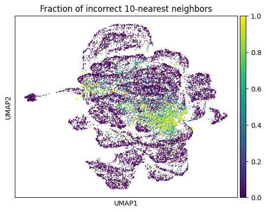
It’s clear from this plot that some areas of the space can be better predicted than others. We can plot the fraction of incorrect labels in the \(k\)-neighborhood of each point.
This tells us exactly where naive \(k\)-NN prediction will fail. However, it can only be computed on a point by using its true label. So we cannot compute it on unlabeled data, and cannot compute it on a test set without test labels.
This is a crucial problem. One way to get around it is to use another measure, like the entropy of the training labels in the neighborhood of each point. But it’s unclear how this would affect test performance of the classifier, or how well this could be estimated over the whole space from training data.
Motivating questions
There are a couple of basic questions we’ll address on test set examples without test labels, in a way we can guarantee can be estimated from training data:
How can we quantify label uncertainty on test examples, in a way that relates to prediction performance on test examples?
How to set the neighborhood size \(k\)?
A prediction algorithm
In the paper (Balsubramani et al. 2019), we introduce a way to view both of these questions. In it, we modify the \(k\)-nearest neighbor prediction rule:
Use fewer neighbors when they all agree about the true label, and more neighbors when there is more uncertainty about the true label.
In areas where there is too much uncertainty, the algorithm will output “?” (“don’t know”).
Setup
For any point \(x\), we speak of:
\(N_k (x)\) as \(x\)’s “k-neighborhood”: a region around \(x\) containing exactly the \(k\) nearest neighbors of \(x\), and no more.
\(\text{bias}_k (x)\) as the bias of the k-neighborhood around \(x\), i.e. the amount by which the frequency of a label exceeds chance.
Prediction rule
Set an abstention parameter \(A > 0\). For a test example \(x\), we predict its label using the \(k^*\) nearest neighbors, where
Use the minimum number of neighbors such that one label occurs significantly more often locally than chance.
We call this rule the Adaptive KNN (AKNN) rule.
Implementation
In practice, we only search over values of \(k\) up to some maximum \(k_{max}\). So AKNN uses \[ k^* (x) = \text{min} \left\{ k \leq
k_{max} : k (\text{bias}_k (x))^2 \geq A^2 \right\} \qquad
\qquad (1) \]
This constraint makes runtime much more reliable. Also, it is natural in practical applications that use approximate \(k\)-NN search, where the accuracy of the search drops as \(k\) increases, e.g. by locality-sensitive hashing.
The code looks like this:
CODE
def aknn(nbrs_arr, labels, thresholds, distinct_labels=['A','B','C','D','E','F','G','H','I','J']):""" Apply AKNN rule for a query point, given its list of nearest neighbors. Parameters ---------- nbrs_arr: array of shape (n_neighbors) Indices of the `n_neighbors` nearest neighbors in the dataset. labels: array of shape (n_samples) Dataset labels. thresholds: array of shape (n_neighbors) Bias thresholds at different neighborhood sizes. Returns ------- pred_label: string AKNN label prediction. first_admissible_ndx: int n-1, where AKNN chooses neighborhood size n. fracs_labels: array of shape (n_labels, n_neighbors) Fraction of each label in balls of different neighborhood sizes. emp_margin: float Empirical "advantage" of the point, as specified by the AKNN paper. """ query_nbrs = labels[nbrs_arr] mtr = np.stack([query_nbrs == i for i in distinct_labels]) rngarr = np.arange(len(nbrs_arr))+1 fracs_labels = np.cumsum(mtr, axis=1)/rngarr biases = fracs_labels -1.0/len(distinct_labels) emp_margin = np.max(rngarr*biases*biases) numlabels_predicted = np.sum(biases > thresholds, axis=0) admissible_ndces = np.where(numlabels_predicted >0)[0] first_admissible_ndx = admissible_ndces[0] iflen(admissible_ndces) >0elselen(nbrs_arr)# Break any ties between labels at stopping radius, by taking the most biased label pred_label ='?'if first_admissible_ndx ==len(nbrs_arr) else distinct_labels[np.argmax(biases[:, first_admissible_ndx])]return (pred_label, first_admissible_ndx, fracs_labels, emp_margin)def predict_nn_rule(nbr_list_sorted, labels, margin=1.0):""" Given matrix of ordered nearest neighbors for each point, returns AKNN's label predictions and adaptive neighborhood sizes. """ pred_labels = [] adaptive_ks = [] emp_margins = [] fracs_labels_list = [] thresholds = margin/np.sqrt(np.arange(nbr_list_sorted.shape[1])+1)for i inrange(nbr_list_sorted.shape[0]): (pred_label, adaptive_k_ndx, fracs_labels, emp_margin) = aknn( nbr_list_sorted[i,:], labels, thresholds, distinct_labels=np.unique(labels)) pred_labels.append(pred_label) adaptive_ks.append(adaptive_k_ndx +1) fracs_labels_list.append(fracs_labels) emp_margins.append(emp_margin)return np.array(pred_labels), np.array(adaptive_ks), np.array(fracs_labels_list), np.array(emp_margins)
A nonparametric margin
The best we can do from a fixed neighborhood
In real situations, neighborhoods around many data of interest will be noisy. This imposes a fundamental limit on how well we can predict in such situations.
If we’re predicting on a point \(x\), suppose a neighborhood around it, containing a fraction \(p\) of the data, has a bias of \(\gamma\). How many points do we need to sample from this neighborhood in order to know that its bias is significantly different from zero?
The answer is clear from basic statistics:
At least \(\Omega (\frac{1}{p \gamma^2})\) samples are required to learn to predict correctly on \(x\) from this neighborhood.
Explanation
Treating the sample labels as biased coin flips, we can answer this by taking a Hoeffding bound: after sampling \(m\) points from the neighborhood, the chance of detecting a bias \(\geq \gamma\) under the null is \(\approx e^{-2 m \gamma^2}\). So the quantity \(m \gamma^2\) measures how easily a significant bias is detected in a neighborhood around \(x\). In practice, \(m\) is proportional to the fraction \(p\) of the data falling in the neighborhood – \(m \approx n p\) – so the quantity we care about for each neighborhood is \(p \gamma^2\).
How many samples are needed to predict correctly near \(x\)? The probability of failure of the Hoeffding bound is \(\leq e^{-2 n p \gamma^2}\); setting this to a fixed failure tolerance \(\delta\), and solving for \(n\), gives \(n = \frac{1}{2 p \gamma^2} \ln (\frac{1}{\delta})\).
Defining a nonparametric margin
Overall, the above discussion tells us that when there is no neighborhood around \(x\) with a low value of \(p \gamma^2\), there is always an unacceptably high chance of incorrectly predicting on \(x\). But any neighborhood around \(x\) with sufficiently high \(p \gamma^2\) can be used to predict correctly on \(x\) from few (\(\Theta (\frac{1}{p \gamma^2})\)) samples.
\(p \gamma^2\) is a purely theoretical quantity, but an empirical version of it is \(k (\text{bias}_k (x))^2\). So the quantity
captures how many examples we need to predict correctly on \(x\).
\(\Gamma\) is high exactly when \(x\) can be correctly predicted by some neighborhood using few examples (high \(p \gamma^2\)). And conversely, \(\Gamma\) is low when all neighborhoods around \(x\) require many examples to learn from (low \(p \gamma^2\)). \(\Gamma\) is a nonparametric version of the margin, which represents how well points can be predicted in the embedding.
Note that in the algorithm implementation we’ve given above, we see that AKNN (x) is simply calculating \(k (\text{bias}_k (x))^2\) and using that to find \(k^* (x)\). Essentially, it is calculating \(\Gamma (x)\) and assigning a label according to the “easiest” data according to \(\Gamma\).
AKNN adapts to nonparametric margin
We introduced a theoretical version of \(\Gamma (x)\) in (Balsubramani et al. 2019), calling it the “advantage” \(\text{adv} (x)\). As I’ve discussed so far, the best this can possibly be for any neighborhood-based method is \(\Omega
\left( \frac{1}{\text{adv} (x)} \right)\). We proved in the main result of (Balsubramani et al. 2019) that with AKNN,
AKNN can learn to predict correctly on any point \(x\) with \(O \left( \frac{1}{\text{adv} (x)} \ln \frac{1}{\text{adv} (x)} \right)\) samples.
So AKNN adapts to the local geometry about as well as possible,1 everywhere in the space at once.
To sum up, we have a notion of nonparametric margin explained from fundamental considerations, and a prediction rule (AKNN) that is well-suited to realize its benefits.
Making the margin meaningful for prediction
To be able to predict well on \(x\), we need to be wary of neighborhoods around \(x\) with high \(p \gamma^2\) that indicate conflicting labels, for instance a point whose immediate closest 1-2 points are weakly negatively biased, within a strongly positive region. In such cases, we would expect A to predict positive, even though the Bayes optimal prediction is negative.
This complicates the empirical picture a little. But we have two saving graces.
This will only happen when the immediate neighborhood is weakly biased, i.e. it is locally noisy. So relative to the Bayes optimal classifier, we would not suffer much more in prediction on those points.
The theory here is very robust, so the major conclusions hold anyway. AKNN as specified is still a well-understood algorithm.
Now that we have an empirical notion of non-parametric margin, we evaluate it across some data.
Experiments with nonparametric margin
Computing nonparametric margin
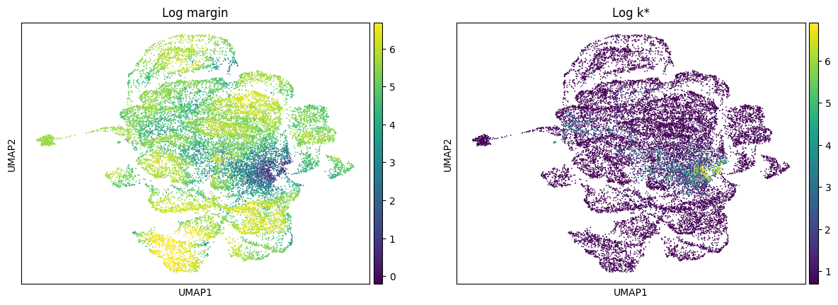
This nonparametric margin isn’t just a neat abstraction to think of local error – it can actually be computed very efficiently.
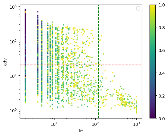
The definition of \(\Gamma (x)\) shows how: this is computable from the neighborhood of \(x\). When this quantity is plotted (in log scale, for ease of visualization), we observe that the low-margin points correspond to those with high required neighborhood sizes.
/var/folders/mn/9bz8ffcj7dj_przhmfwl3b5h0000gn/T/ipykernel_49510/3607783998.py:6: UserWarning: No artists with labels found to put in legend.  Note that artists whose label start with an underscore are ignored when legend() is called with no argument.
  plt.legend()
The dotted lines illustrate the following conclusions:
Examples with a high empirical margin (above the red dotted line), which are “easy” to learn, have relatively low adaptive \(k\) - it’s not necessary to choose a high adaptive \(k\) to cover them.
Examples with high adaptive \(k\) (right of the green dotted line) all have low empirical margin (they are “hard,” below the red dotted line). So if we’ve used little data and \(n\) is small, it makes sense to abstain upon them.
CODE
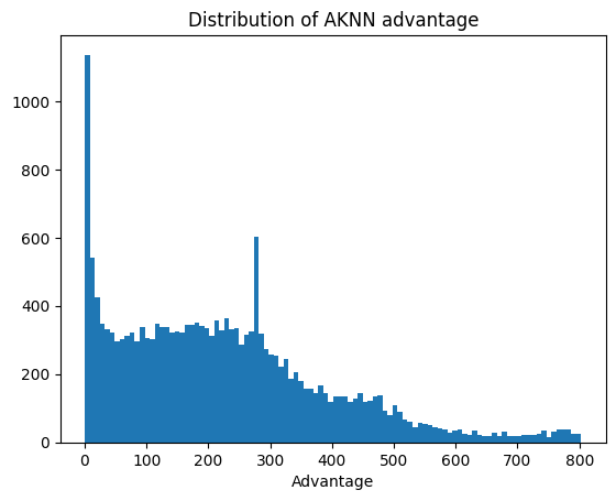
plt.hist(aknn_predictions[3], bins=100)#.value_counts()plt.xlabel("Advantage")plt.title("Distribution of AKNN advantage")plt.show()
Speeding up the implementation
The main flaw with this implementation is that every query point requires its own function call. It is far preferable to have a vectorized implementation, which can batch-wise amortize the thresholding and averaging operations required to run AKNN.
CODE
def predict_nn_rule_vectorized(nbr_list_sorted, labels, margin_param=1.0):""" Apply AKNN rule for a query point, given its list of nearest neighbors. Parameters ---------- nbrs_arr: array of shape (n_queries, n_neighbors) Indices of the `n_neighbors` nearest neighbors in the dataset, for each query point. labels: array of shape (n_samples,) Dataset labels, for the full dataset from which the neighbors were selected. margin_param: float The confidence parameter for the AKNN rule. Returns ------- pred_label: array of shape (n_queries,) AKNN label predictions. first_admissible_ndx: array of shape (n_queries,) The first admissible neighborhood size for each query point. 0 means no admissible neighborhood size. n-1 means AKNN chooses neighborhood size n. fracs_labels: array of shape (n_queries, n_labels, n_neighbors) For each query point, the fraction of each label in balls of different neighborhood sizes. emp_margins: array of shape (n_queries,) Empirical "advantage" of each query point, as specified by the AKNN paper. """ distinct_labels = np.unique(labels) num_data, K = nbr_list_sorted.shape num_labels =len(distinct_labels) thresholds = margin_param/np.sqrt(np.arange(1,K+1)) code_by_sample = np.searchsorted(distinct_labels, labels) nbr_codes = code_by_sample[nbr_list_sorted] # (Q,K) mtr = (nbr_codes[:,None,:] == np.arange(num_labels)[None,:,None]).astype(np.int32) # (Q,L,K) fracs_labels = np.cumsum(mtr, axis=2)/np.arange(1, K+1)[None, None, :] # (Q,L,K) biases = fracs_labels - (1.0/num_labels) emp_margins = np.max(np.arange(1, K+1)[None, None, :]*biases*biases, axis=(1,2)) admissible = np.sum(biases > thresholds[None, None, :], axis=1) >0# (Q,K) bool has_adm = np.any(admissible, axis=1) first_ndx = np.argmax(admissible, axis=1) # 0..K-1 (or 0 if none) idx_k = np.clip(first_ndx, 0, K-1)[:, None, None] b_at_k = np.take_along_axis(biases, idx_k, axis=2)[:, :, 0] # (Q,L) best_code = b_at_k.argmax(axis=1) pred_labels = np.full(num_data,'?',dtype=object) pred_labels[has_adm] = distinct_labels[best_code[has_adm]] adaptive_ks = np.where(has_adm, first_ndx+1, K+1) # +1; K+1 means “no stop”return pred_labels, adaptive_ks, fracs_labels, emp_margins
87.1 ms ± 7.05 ms per loop (mean ± std. dev. of 7 runs, 10 loops each)
This speedup is significant (at least 3x) even at such small scales.
Related work
Other work
There’s a lengthy discussion of the history of kNN work in the paper (Balsubramani et al. 2019). To summarize it here, a long line of work culminating in (Chaudhuri and Dasgupta 2014) gives a tight understanding of the convergence rate of the “vanilla” kNN prediction rule, which uses the same \(k\) everywhere. Different regions of space have different convergence rates for kNN, so “local” understanding is a vital part of this picture.
Building on this understanding, we introduced a nonparametric local notion of margin, the “advantage,” which we computed efficiently and found to be a useful number to plot. This sets a theoretical performance limit that’s dependent on the properties of the embedded data, but not on any parametric model. And in AKNN, we give a rule that adapts to the advantage at any point and optimally realizes the performance quantified by the advantage.
Open problems
Our main focus in this post has been trying to operationally define “easy” and “hard” data and empirically explore what these mean in real data. Nonparametric classification gives a wonderful, model-free way to explore these notions. Our nonparametric notion of margin (the “advantage”) gives a tight local understanding of how hard it is to predict on a point from its neighborhood. The AKNN algorithm that complements it provably adapts to this local advantage, only requiring “as many labels as necessary.”
This opens up new questions:
Can this local margin be used for active learning? Uncertainty estimation?
Can AKNN be adapted to active or distributed settings?
The notion of nonparametric margin we have here can be robustified and extended as well. It’s fundamental and demonstrably empirically versatile, and is a good building block for further analysis of embeddings.
References
Aumüller, Martin, Erik Bernhardsson, and Alexander Faithfull. 2020. “ANN-Benchmarks: A Benchmarking Tool for Approximate Nearest Neighbor Algorithms.”Information Systems 87: 101374.
Balsubramani, Akshay, Sanjoy Dasgupta, Yoav Freund, and Shay Moran. 2019. “An Adaptive Nearest Neighbor Rule for Classification.”Advances in Neural Information Processing Systems 32.
Chaudhuri, Kamalika, and Sanjoy Dasgupta. 2014. “Rates of Convergence for Nearest Neighbor Classification.”Advances in Neural Information Processing Systems 27.
Eaton, Morris L. 1989. “Group Invariance Applications in Statistics.” In. IMS.
Sidak, Zbynek, Pranab K Sen, and Jaroslav Hajek. 1999. Theory of Rank Tests. Elsevier.
Stone, Charles J. 1977. “Consistent Nonparametric Regression.”The Annals of Statistics, 595–620.
Wijsman, Robert A. 1990. “Invariant Measures on Groups and Their Use in Statistics.” In. IMS.
Footnotes
In practice, the embeddings are themselves learned, so Euclidean geometry is typically the one the matters. But the method and theory go well beyond Euclidean geometry, and the results hold unchanged for any metric space that behaves smoothly locally, i.e., any metric space in which the Fundamental Theorem of Calculus holds. See Theorem 4 from (Balsubramani et al. 2019).↩︎