The fundamental ideas underpinning modern AI and machine learning involve recognition of statistical patterns from sampled training data, which generalize usefully to a test-time setting. The basic probabilistic questions involved here are universal:
How much can be learned about a probability distribution from a finite sample of it?
What happens when the test-time distribution being evaluated is different from the training distribution?
Which patterns and representations usefully generalize to other distributions and datasets?
To begin understanding these basic principles of machine learning, it can be useful to understand concentration of samples from a distribution. This understanding has been put together progressively over time. The story is related to the origins of the field, but goes much further back, to the heart of probability and information theory. It is also central to statistical mechanics, a field studying the collective (macroscopic) behavior of large populations of (microscopic) atoms.
In the late 19th century, as scientists tried to relate properties of bulk matter to its individual atoms, they sought a quantitative theory of this collective behavior. Development of the field was stalled at a basic level of understanding for many decades, in which unexplained observations were plentiful and unifying explanations scarce - the problem was daunting, because of the huge numbers of microscopic entities involved.
Progress came from a revolutionary insight by Boltzmann. When he considered a discretized probability-calculation scenario in 1877 (see , trans. ), he launched the field of statistical mechanics . The argument he used is extremely foundational in an AI context even today, when models learned by loss minimization, like deep neural networks, dominate.
Here’s an overview of Boltzmann’s core statistical mechanics understanding. With this entry point, we can ultimately describe modern-day (loss-minimization-based) AI modeling in statistical mechanics terms. This particular link between modeling and statistical mechanics is foundational, and contains many basic insights into models. It allows us to see the essential unity between the basic concepts underlying loss minimization, information theory, and statistical physics.
Concentration
Start with the first basic question from earlier: How much can be learned about a probability distribution from a finite sample of it? In probability theory terms, given a distribution \(P\) over a set of outcomes \(\mathcal{X}\), we are looking to understand the consequences of repeatedly sampling from \(P\). Boltzmann’s insight was that if the set of outcomes \(\mathcal{X}\) is finite, this question can be tractably answered by explicitly counting the possibilities. Suppose \(\mathcal{X}\) is finite: \(\mathcal{X} = \{x_1, x_2, \dots, x_D \}\). We draw \(n\) samples from this set independently according to a probability distribution \(P = (P_1, \dots, P_D)\), and we observe the frequencies of each outcome. Let \(n_i\) be the number of times we observe outcome \(x_i\), so that \(\sum_{i} n_{i} = n\). The observed probability of outcome \(x_i\) is then \(Q_i := n_i / n\), so \(Q\) is another probability distribution over \(\mathcal{X}\). Boltzmann calculated the probability of observing a particular set of frequencies \(\{n_1, \dots, n_D\}\) in this situation: \[
\begin{aligned}
\frac{1}{n} \log \text{Pr} (x_1 = n_1, \dots, x_D = n_D)
&= - \text{D} (Q \mid \mid P ) + \frac{1}{2 n} \log \left( \frac{2 \pi n}{ \prod_{i=1}^{D} (2 \pi n P_i) } \right) + \Theta (1 / n^2) \\
\end{aligned}
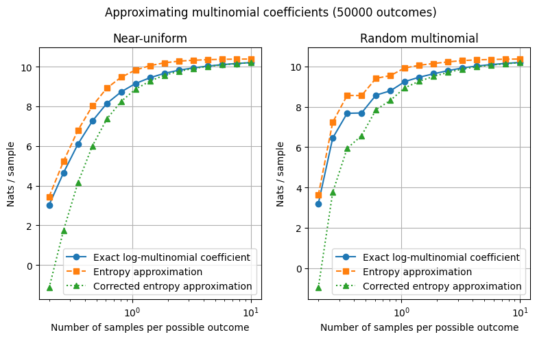
\] This is an extremely accurate and powerful approximation for even moderate sample sizes \(n\), which tells us the likelihood of observing any specific configuration of outcomes.
We’ve calculated the chance of observing a particular set of frequencies given \(P\).
The real distribution \(P\) only enters the picture through its divergence from the observed distribution \(Q\). This \(- \text{D} (Q \mid \mid P )\) is also by far the dominant term, as all the others are \(O(1/n)\).
In short, observing the histogram \(Q\) alone does not determine \(P\), but it does give us enough information to precisely quantify the likelihood of deviations of \(Q\) from \(P\).
Boltzmann’s probability calculation
Boltzmann’s proof is the most direct one even after over a century, and it is well worth recapitulating. Discretizing the probability space, and discretizing quanta of probability (at resolution \(\frac{1}{n}\)), gives essentially a generalized balls-in-bins problem, which Boltzmann solved. The calculation is simply a matter of accounting for the differently weighted “bins” (outcomes), and the combinatorially many ways of throwing “balls” (quanta of probability) into them.
\[\begin{align*}
\text{Pr} (x_1 = n_1, \dots, x_D = n_D)
&= \frac{n!}{n_1! \cdots n_D!} Q_1^{n_1} \cdots Q_D^{n_D} \\
&= \frac{n!}{n_1! \cdots n_D!} \exp \left( n_1 \log Q_1 + \cdots + n_D \log Q_D \right) \\
&= \frac{n!}{(n P_1)! \cdots (n P_D)!} \exp \left( n \sum_{i=1}^{D} P_i \log Q_i \right) \\
&= \frac{n!}{(n P_1)! \cdots (n P_D)!} \exp \left( - n \text{H} (P, Q) \right)
\end{align*}\] We can rewrite the multinomial coefficient using Stirling’s approximation ($ n! = n n - n + (2 n) + (1/n) \().\)\(\begin{align*}
\log \left( \frac{n!}{(n P_1)! \cdots (n P_D)!} \right)
&= n \log n - n + \frac{1}{2} \log (2 \pi n) - \sum_{i=1}^{D} \left[ n P_i \log n P_i - n P_i + \frac{1}{2} \log (2 \pi n P_i) \right] + \Theta (1/n) \\
&= n \log n + \frac{1}{2} \log (2 \pi n) - n \sum_{i=1}^{D} P_i \log n P_i - \frac{1}{2} \sum_{i=1}^{D} \log (2 \pi n P_i) + \Theta (1/n) \\
&= n \text{H} (P) + \frac{1}{2} \log (2 \pi n) - \frac{1}{2} \sum_{i=1}^{D} \log (2 \pi n P_i) + \Theta (1/n)
\end{align*}\)$ Therefore, the probability of observing the frequencies \(n_1, \dots, n_D\) is \[
\begin{aligned}
\text{Pr} (x_1 = n_1, \dots, x_D = n_D)
&= \exp \left( - n \sum_{i=1}^{D} P_i \log \frac{P_i}{Q_i} + \frac{1}{2} \log \left( \frac{2 \pi n}{ \prod_{i=1}^{D} (2 \pi n P_i) } \right) + \Theta (1/n) \right)
\end{aligned}
\] Restating this gives the result.
Impact and consequences
What Boltzmann called his ``probability calculations” () launched the field of statistical mechanics, and inspired the field of information theory decades later. This is because discretizing the space is a fully general technique, containing all the essential elements used to study concentration and collective behavior in statistical mechanics.
The calculation shows the degeneracy in observing the histogram \(Q\) - the “macrostate” of the \(n\)-sample dataset - from a particular “microstate,” i.e. the individual outcomes of each of the \(n\) samples. This was the idea that allowed physicists to quantify observable bulk properties of matter (macrostates) from unobservable configurations of each of its atoms (microstates).
In AI and data science, the system being studied (the “matter”) is a dataset comprising examples, whose state is the microstate. And the macrostate consists of our coarse-grained observations about the dataset, as we develop more in the following sections.
This multinomial coefficient is the number of ways to get the same observed macrostate (the histogram \(Q\)) from particular microstates (the individual values of all the examples in the dataset). In other words, microstates can be counted in terms of the entropy of the observed macrostate.
Putting all this together, we arrive at some powerful insights.
Entropy is a measure of the microscopic multiplicity, or degeneracy, associated with a set of limited macroscopic/average observations into the underlying microstate. High-entropy configurations are exponentially more likely than other configurations - they dominate observed configurations for large \(n\).
Therefore, the macrostate maximizing entropy is the “most likely” state. Entropy maximization accounts for the many microstates that are consistent with a set of macroscopic observations.
In the macroscopically sized samples of atoms we observe in everyday life, our observations are almost deterministic, even of highly disordered systems like gaseous and liquid matter. This is because they are made of moles of individual constituents, and our handful of bulk properties observed about them corresponds to only a handful of constraints.
In the statistical mechanical view of AI, when trying to minimize loss over datasets, we can similarly say that the entropy of the learned distribution tends to be nearly maximal. (This can be proved quite generally.)
What we’ve described, with a discrete “alphabet” of possible states, is the concept called the asymptotic equipartition property in information theory – high-entropy sequences occur with much greater multiplicity than low-entropy ones. Boltzmann’s “probability calculation” shows exactly why, with entropy emerging as a measure of (log) multiplicity.