Foundations of concentration and entropy

statmech

Where entropy comes from

Author

Akshay Balsubramani

Published

July 23, 2024

Modified

August 19, 2024

Foundations: entropy, concentration, and learning

The fundamental ideas underpinning modern AI and machine learning involve recognition of statistical patterns from sampled training data, which generalize usefully to a test-time setting. The basic probabilistic questions involved here are universal:

How much can be learned about a probability distribution from a finite sample of it?
What happens when the test-time distribution being evaluated is different from the training distribution?
Which patterns and representations usefully generalize to other distributions and datasets?

To begin understanding these basic principles of machine learning, we need to understand concentration of samples from a distribution. This understanding has been put together progressively over time. The story is related to the origins of the field, but goes much further back, to the heart of probability and information theory. It is also central to statistical mechanics, a field studying the collective (macroscopic) behavior of large populations of (microscopic) atoms.

In the late 19th century, as scientists tried to relate properties of bulk matter to its individual atoms, they sought a quantitative theory of this collective behavior. Development of the field was stalled at a basic level of understanding for many decades, in which unexplained observations were plentiful and unifying explanations scarce - the problem was daunting, because of the huge numbers of microscopic entities involved.

Progress came from a revolutionary insight by Boltzmann. When he considered a discretized probability-calculation scenario in 1877 (see , trans. ), he launched the field of statistical mechanics . The argument he used is extremely foundational in an AI context even today, when models learned by loss minimization, like deep neural networks, dominate.

So we explore Boltzmann’s core statistical mechanics understanding in detail. With this entry point, we ultimately describe modern-day (loss-minimization-based) AI modeling in statistical mechanics terms. This particular link between modeling and statistical mechanics is foundational, and contains many basic insights into models. It allows us to see the essential unity between the basic concepts underlying loss minimization, information theory, and statistical physics.

Context among related work

Starting from Boltzmann, the history of these ideas is long and vast. It goes back to their discovery in physics in the early 20th century, and many of these concepts are well-known in modern ML as well. Here is a brief discussion - more detailed elaboration will be in the notes.

As we have stated, these ideas have a long history in the statistical mechanics of Boltzmann and Gibbs. In the postwar years of the 1940s, the basics resurfaced for discrete alphabets with the flowering of information theory. The engineering focus of the field, with advances built on semiconductor advances in computing, resulted in a different approach and focus to areas such as coding and processing of probabilistic uncertainty (information).

These ideas were being developed in statistics as well, by Fisher and many others . The different focus there is reflected in the primary role of “exponential families,” particularly for certain types of statistics. Interestingly, it took longer to appreciate the connections between this branch of statistics and the ongoing work in information theory. Methods of information geometry have more recently developed around some of these ideas.

Presently, many ML researchers are aware of these ideas through their appearance in “energy-based models” (EBMs ), which take the energy function of a Gibbs ensemble as a starting point for modeling. EBMs are a key part of the modern deep learning toolkit, as a class of models for which a wide range of interpretations and tools is available.

For EBMs, the connections between the learning loss-minimization perspective and the statistical mechanics perspective are applied by formal analogy , as a way to avoid dealing with a probability-normalization constraint. The model class and distribution are typically given a priori, without using max-entropy or the observation constraints associated with the energy function. Works like use statistical mechanics notions like energy and temperature as powerful tools to analyze black-box computation .

Our purpose here is to center this view (see ), allowing us to elucidate the stat-mech view of prediction in full generality.

Scope

The purpose here is to comprehensively lay out the statistical mechanics view of loss minimization scenarios. Such scenarios are everywhere in modern AI systems. This viewpoint enables us to cross-fertilize ideas between our world of data modeling on one hand, and statistical physics and information theory on the other.

For the most part, these are well-established concepts that do not require complex technical machinery to handle real-world modeling scenarios. So we will prove many general results, but with as little needed technically as possible. Self-contained derivations of these results are helpful for several reasons:

The results have well-understood interpretations in the real world, as describing the behavior of bulk observed properties emerging from simply applying some basic underlying principles. These interpretations can be translated into data-modeling situations.
The methods used for the derivations, from optimization, game theory, and convexity, are familiar tools to AI researchers. But in the context of the results in physics and information theory, they lead to sometimes nonstandard derivations of known results. And these derivations’ broad scope and applicability, to new problems and loss functions, gives the results significant new power, significantly broadening their applications.
Following developments in AI and modeling, the powerful results of physics and information theory can be extended: to new models, systems with size/regularization which do not occur in observable physics, and more.

Concentration: Boltzmann’s probability calculation

Start with the first basic question from earlier: How much can be learned about a probability distribution from a finite sample of it?

In probability theory terms,
given a distribution $P$ over a set of outcomes $\mathcal{X}$, we are looking to understand the consequences of repeatedly sampling from $P$. Boltzmann’s insight was that if the set of outcomes $\mathcal{X}$ is finite, this question can be tractably answered by explicitly counting the possibilities.

Suppose $\mathcal{X}$ is finite: $\mathcal{X} = \{x_1, x_2, \dots, x_D \}$. We draw $n$ samples from this set independently according to a probability distribution $P = (P_1, \dots, P_D)$, and we observe the frequencies of each outcome. Let $n_i$ be the number of times we observe outcome $x_i$, so that $\sum_{i} n_{i} = n$. The observed probability of outcome $x_i$ is then $Q_i := n_i / n$, so $Q$ is another probability distribution over $\mathcal{X}$.

Boltzmann calculated the probability of observing a particular set of frequencies $\{n_1, \dots, n_D\}$ in this situation: \[ \begin{aligned} \frac{1}{n} \log \text{Pr} (x_1 = n_1, \dots, x_D = n_D) &= - \text{D} (Q \mid \mid P ) + \frac{1}{2 n} \log \left( \frac{2 \pi n}{ \prod_{i=1}^{D} (2 \pi n P_i) } \right) + \Theta (1 / n^2) \\ \end{aligned} \]

This is an extremely accurate and powerful approximation for even moderate sample sizes $n$, which tells us the likelihood of observing any specific configuration of outcomes.

We’ve calculated the chance of observing a particular set of frequencies given $P$.
The real distribution $P$ only enters the picture through its divergence from the observed distribution $Q$. This $- \text{D} (Q \mid \mid P )$ is also by far the dominant term, as all the others are $O(1/n)$.

In short, observing the histogram $Q$ alone does not determine $P$, but it does give us enough information to precisely quantify the likelihood of deviations of $Q$ from $P$.

Proof

Boltzmann’s proof is the most direct one even after over a century, and it is well worth recapitulating. Discretizing the probability space, and discretizing quanta of probability (at resolution $\frac{1}{n}$), gives essentially a generalized balls-in-bins problem, which Boltzmann solved. The calculation is simply a matter of accounting for the differently weighted “bins” (outcomes), and the combinatorially many ways of throwing “balls” (quanta of probability) into them.

$\textbf{Proof}$

\[\begin{align*} \text{Pr} (x_1 = n_1, \dots, x_D = n_D) &= \frac{n!}{n_1! \cdots n_D!} Q_1^{n_1} \cdots Q_D^{n_D} \\ &= \frac{n!}{n_1! \cdots n_D!} \exp \left( n_1 \log Q_1 + \cdots + n_D \log Q_D \right) \\ &= \frac{n!}{(n P_1)! \cdots (n P_D)!} \exp \left( n \sum_{i=1}^{D} P_i \log Q_i \right) \\ &= \frac{n!}{(n P_1)! \cdots (n P_D)!} \exp \left( - n \text{H} (P, Q) \right) \end{align*}\]

We can rewrite the multinomial coefficient using Stirling’s approximation ($ n! n n - n + (2 n) + (1/n) $).

\[\begin{align*} \log \left( \frac{n!}{(n P_1)! \cdots (n P_D)!} \right) &= n \log n - n + \frac{1}{2} \log (2 \pi n) - \sum_{i=1}^{D} \left[ n P_i \log n P_i - n P_i + \frac{1}{2} \log (2 \pi n P_i) \right] + \Theta (1/n) \\ &= n \log n + \frac{1}{2} \log (2 \pi n) - n \sum_{i=1}^{D} P_i \log n P_i - \frac{1}{2} \sum_{i=1}^{D} \log (2 \pi n P_i) + \Theta (1/n) \\ &= n \text{H} (P) + \frac{1}{2} \log (2 \pi n) - \frac{1}{2} \sum_{i=1}^{D} \log (2 \pi n P_i) + \Theta (1/n) \end{align*}\]

Therefore, the probability of observing the frequencies $n_1, \dots, n_D$ is \[ \begin{aligned} \text{Pr} (x_1 = n_1, \dots, x_D = n_D) &= \exp \left( - n \sum_{i=1}^{D} P_i \log \frac{P_i}{Q_i} + \frac{1}{2} \log \left( \frac{2 \pi n}{ \prod_{i=1}^{D} (2 \pi n P_i) } \right) + \Theta (1/n) \right) \\ \end{aligned} \]

Restating this gives the result.

Impact and consequences

What Boltzmann called his ``probability calculations” () launched the field of statistical mechanics, and inspired the field of information theory decades later. This is because discretizing the space is a fully general technique, containing all the essential elements used to study concentration and collective behavior in statistical mechanics.

The calculation shows the degeneracy in observing the histogram $Q$ - the “macrostate” of the $n$-sample dataset - from a particular “microstate,” i.e. the individual outcomes of each of the $n$ samples. This was the idea that allowed physicists to quantify observable bulk properties of matter (macrostates) from unobservable configurations of each of its atoms (microstates).

In AI and data science, the system being studied (the “matter”) is a dataset comprising $n$ examples, whose state is the microstate. And the macrostate consists of our coarse-grained observations about the dataset, as we develop more in the following sections.

Enter entropy

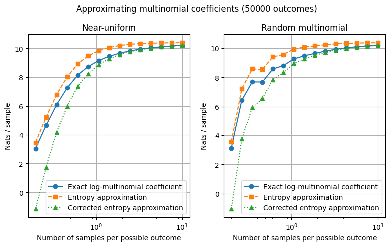
In this calculation, the log-multinomial coefficient $\log \left( \frac{n!}{(n P_1)! \cdots (n P_D)!} \right)$ is $\approx n \text{H} (P)$, with the approximation being very accurate for even moderate $n$. In fact, this is the only approximation that we have made in the calculation. How accurate is it?

We can quantify the relative accuracy, i.e. the difference between the log-multinomial coefficient and $n \text{H} (P)$, EXPONENTIATED. Do this for different $P$ (and $D$), and plot it vs. $n$. Note that even for moderate $n$, the relative error is <1%.

CODE

import numpy as np
from scipy.special import binom, gammaln
from scipy.stats import entropy, dirichlet
import matplotlib.pyplot as plt
import time

def log_multinomial(freqs):
    if len(freqs) == 1:
        return 0
    # corrected_freqs = freqs #np.maximum(freqs, 1)   # Convert 0s to 1s
    cumsum = 0
    for i in range(len(freqs)):
        these_freqs = freqs[:len(freqs)-i]
        cumsum += log_binomial(sum(these_freqs), these_freqs[-1])
    return cumsum

# A function for computing np.log(n!/k!(n-k)!)
def log_binomial(n, k):
    if k==0:
        return 0
    log_binom = gammaln(n+1) - gammaln(k+1) - gammaln(n-k+1)
    return log_binom

def correction_term(freqs):
    n = np.sum(freqs)
    corrected_freqs = np.maximum(freqs, 1)   # Convert 0s to 1s
    return 0.5*(np.log(2*np.pi*n) - np.sum(np.log(2*np.pi*corrected_freqs)))


def return_approximations(test_distribution, n_values):
    exact_values = []
    approx_values = []
    corrected_values = []
    itime = time.time()
    for n in n_values:
        freqs = np.squeeze(np.round(n*test_distribution))

        logmult = log_multinomial(freqs)
        print('*', time.time()-itime)
        entropy_approx = (np.sum(freqs))*entropy(freqs/np.sum(freqs))
        print('**', time.time() - itime)
        corrected_approx = entropy_approx + correction_term(freqs)
        print('***', time.time()-itime)

        exact_values.append(logmult*(1.0/n))
        approx_values.append(entropy_approx*(1.0/n))
        corrected_values.append(corrected_approx*(1.0/n))

        results_str = "Log multinomial coefficient (n = {}): {:.2f} \nEntropy approximation: {:.2f} \nCorrected approximation error: {:.4f}\n".format(
            n, 
            logmult, 
            entropy_approx, 
            corrected_approx
        )
        print(results_str)
    return exact_values, approx_values, corrected_values

CODE

num_outcomes = 50000

# Simulate a multinomial distribution from a Dirichlet distribution
n_values = np.geomspace(num_outcomes*0.2, num_outcomes*10, 15).astype(int)

alpha = np.ones(num_outcomes)
test_distribution_unif = dirichlet.rvs(alpha, size=1, random_state=42)

distr = np.random.rand(num_outcomes)
test_distribution_mult = np.square(distr/np.linalg.norm(distr))

exact_values_unif, approx_values_unif, corrected_values_unif = return_approximations(test_distribution_unif, n_values)
exact_values_mult, approx_values_mult, corrected_values_mult = return_approximations(test_distribution_mult, n_values)

* 61.577237129211426
** 61.57803916931152
*** 61.57839012145996
Log multinomial coefficient (n = 10000): 30337.26 
Entropy approximation: 34457.23 
Corrected approximation error: -11492.5833

* 124.60214519500732
** 124.60284185409546
*** 124.60320687294006
Log multinomial coefficient (n = 13223): 61547.20 
Entropy approximation: 69163.83 
Corrected approximation error: 23157.9197

* 184.47993922233582
** 184.48086500167847
*** 184.48120188713074
Log multinomial coefficient (n = 17486): 106644.15 
Entropy approximation: 118807.16 
Corrected approximation error: 72614.7712

* 246.3503770828247
** 246.35137701034546
*** 246.3516948223114
Log multinomial coefficient (n = 23124): 167866.46 
Entropy approximation: 185425.25 
Corrected approximation error: 138755.5875

* 308.3903560638428
** 308.39125418663025
*** 308.3915379047394
Log multinomial coefficient (n = 30578): 249107.63 
Entropy approximation: 272701.01 
Corrected approximation error: 225057.7763

* 370.4352550506592
** 370.43617010116577
*** 370.4364891052246
Log multinomial coefficient (n = 40436): 353073.85 
Entropy approximation: 382948.34 
Corrected approximation error: 333710.4028

* 430.1966769695282
** 430.19748306274414
*** 430.1977469921112
Log multinomial coefficient (n = 53472): 489503.28 
Entropy approximation: 525866.67 
Corrected approximation error: 474289.1029

* 490.84602093696594
** 490.8472001552582
*** 490.84748005867004
Log multinomial coefficient (n = 70710): 667751.78 
Entropy approximation: 710701.25 
Corrected approximation error: 656041.8695

* 551.4618928432465
** 551.4626441001892
*** 551.4629120826721
Log multinomial coefficient (n = 93506): 903786.78 
Entropy approximation: 953419.10 
Corrected approximation error: 894951.6779

* 612.1427049636841
** 612.1436381340027
*** 612.1440191268921
Log multinomial coefficient (n = 123650): 1214624.86 
Entropy approximation: 1270965.67 
Corrected approximation error: 1208076.5294

* 671.6361320018768
** 671.6368389129639
*** 671.6371059417725
Log multinomial coefficient (n = 163512): 1625147.14 
Entropy approximation: 1688154.66 
Corrected approximation error: 1620307.7373

* 732.3417410850525
** 732.3424370288849
*** 732.3427059650421
Log multinomial coefficient (n = 216224): 2168945.49 
Entropy approximation: 2238649.68 
Corrected approximation error: 2165386.0623

* 793.2725918292999
** 793.2735450267792
*** 793.2738180160522
Log multinomial coefficient (n = 285930): 2889129.35 
Entropy approximation: 2965642.38 
Corrected approximation error: 2886610.8010

* 855.4713549613953
** 855.4720211029053
*** 855.472284078598
Log multinomial coefficient (n = 378107): 3841814.35 
Entropy approximation: 3925109.05 
Corrected approximation error: 3840036.5819

* 916.2100429534912
** 916.2107310295105
*** 916.2109980583191
Log multinomial coefficient (n = 500000): 5103202.81 
Entropy approximation: 5193286.47 
Corrected approximation error: 5101957.4502

* 60.48375391960144
** 60.48431181907654
*** 60.4845769405365
Log multinomial coefficient (n = 10000): 31187.28 
Entropy approximation: 35423.18 
Corrected approximation error: -10518.6484

* 122.45046877861023
** 122.4511890411377
*** 122.45145869255066
Log multinomial coefficient (n = 13223): 85172.23 
Entropy approximation: 95498.69 
Corrected approximation error: 49557.3017

* 181.6340458393097
** 181.63516187667847
*** 181.6354398727417
Log multinomial coefficient (n = 17486): 134454.62 
Entropy approximation: 149989.87 
Corrected approximation error: 104048.6917

* 242.6539180278778
** 242.6547348499298
*** 242.65499901771545
Log multinomial coefficient (n = 23124): 177550.81 
Entropy approximation: 197491.94 
Corrected approximation error: 151550.8792

* 303.28152775764465
** 303.28238701820374
*** 303.2826509475708
Log multinomial coefficient (n = 30578): 262117.13 
Entropy approximation: 287517.62 
Corrected approximation error: 239956.5123

* 363.8782789707184
** 363.8793270587921
*** 363.8796019554138
Log multinomial coefficient (n = 40436): 356035.63 
Entropy approximation: 386658.12 
Corrected approximation error: 336996.2229

* 424.42981791496277
** 424.4310300350189
*** 424.4313049316406
Log multinomial coefficient (n = 53472): 495234.94 
Entropy approximation: 531522.49 
Corrected approximation error: 478905.1699

* 486.7965009212494
** 486.7976870536804
*** 486.7979657649994
Log multinomial coefficient (n = 70710): 670157.52 
Entropy approximation: 712113.80 
Corrected approximation error: 656152.6677

* 546.0931100845337
** 546.0941939353943
*** 546.0944678783417
Log multinomial coefficient (n = 93506): 901574.47 
Entropy approximation: 949339.59 
Corrected approximation error: 889508.1982

* 609.6344840526581
** 609.6352188587189
*** 609.6354808807373
Log multinomial coefficient (n = 123650): 1211469.52 
Entropy approximation: 1265151.15 
Corrected approximation error: 1201045.1913

* 673.2467420101166
** 673.247475862503
*** 673.247752904892
Log multinomial coefficient (n = 163512): 1622813.02 
Entropy approximation: 1682554.77 
Corrected approximation error: 1613801.0259

* 734.1121428012848
** 734.1129238605499
*** 734.1131930351257
Log multinomial coefficient (n = 216224): 2166387.70 
Entropy approximation: 2232270.41 
Corrected approximation error: 2158563.3091

* 794.8526017665863
** 794.8537039756775
*** 794.8539838790894
Log multinomial coefficient (n = 285930): 2887303.96 
Entropy approximation: 2959476.58 
Corrected approximation error: 2880537.9915

* 854.5094380378723
** 854.5101850032806
*** 854.5104520320892
Log multinomial coefficient (n = 378107): 3837781.18 
Entropy approximation: 3916305.30 
Corrected approximation error: 3831938.2554

* 917.2488069534302
** 917.2495839595795
*** 917.2498650550842
Log multinomial coefficient (n = 500000): 5100082.21 
Entropy approximation: 5185034.53 
Corrected approximation error: 5095028.0008

CODE

# Plotting
absc = n_values/num_outcomes

fig, axs = plt.subplots(1, 2, figsize=(8, 5))
axs[0].set_xscale('log')
axs[0].plot(absc, exact_values_unif, label='Exact log-multinomial coefficient', marker='o')
axs[0].plot(absc, approx_values_unif, label='Entropy approximation', linestyle='--', marker='s')
axs[0].plot(absc, corrected_values_unif, label='Corrected entropy approximation', linestyle=':', marker='^')
axs[0].set_xlabel('Number of samples per possible outcome')
axs[0].set_ylabel('Nats / sample')
axs[0].title.set_text('Near-uniform')
axs[0].legend()
axs[0].grid(True)

axs[1].set_xscale('log')
axs[1].plot(absc, exact_values_mult, label='Exact log-multinomial coefficient', marker='o')
axs[1].plot(absc, approx_values_mult, label='Entropy approximation', linestyle='--', marker='s')
axs[1].plot(absc, corrected_values_mult, label='Corrected entropy approximation', linestyle=':', marker='^')
axs[1].set_xlabel('Number of samples per possible outcome')
axs[1].set_ylabel('Nats / sample')
axs[1].title.set_text('Random multinomial')
axs[1].legend()
axs[1].grid(True)

fig.suptitle(f'Approximating multinomial coefficients ({num_outcomes} outcomes)')
plt.tight_layout()
plt.show()
fig.savefig(f'multinomial_approximations_{num_outcomes}.png', dpi=300)

This multinomial coefficient is the number of ways to get the same observed macrostate (the histogram $Q$) from particular microstates (the individual values of all the examples in the dataset). In other words, microstates can be counted in terms of the entropy of the observed macrostate.

Putting all this together, we arrive at some powerful insights.

Entropy is a measure of the microscopic multiplicity, or degeneracy, associated with a set of limited macroscopic/average observations into the underlying microstate. High-entropy configurations are exponentially more likely than other configurations - they dominate observed configurations for large $n$.
Therefore, the macrostate maximizing entropy is the “most likely” state. Entropy maximization accounts for the many microstates that are consistent with a set of macroscopic observations.

In the macroscopically sized samples of atoms we observe in everyday life, our observations are almost deterministic, even of highly disordered systems like gaseous and liquid matter. This is because they are made of moles of individual constituents, and our handful of bulk properties observed about them corresponds to only a handful of constraints.

In the statistical mechanical view of AI, when trying to minimize loss over datasets, we can similarly say that the entropy of the learned distribution tends to be nearly maximal. (We later prove this, in a very general sense.)

What we’ve described, with a discrete “alphabet” of possible states, is the concept called the asymptotic equipartition property in information theory – high-entropy sequences occur with much greater multiplicity than low-entropy ones (Cover and Thomas 2006). Boltzmann’s “probability calculation” shows exactly why, with entropy emerging as a measure of (log) multiplicity.

References

Cover, Thomas M, and Joy A Thomas. 2006. Elements of Information Theory. Wiley-Interscience.