CODE
# If needed:
# !pip -q install datasets transformers torch torchvision torchaudio scikit-learn --upgrade
# !pip -q install detoxify==0.5.2
# !pip -q install matplotlibIn many situations in AI and LLM evaluation, imbalanced classification problems occur because the things we care about are rare by design. Safety violations, credible threats, medical red flags, jailbreak attempts, code vulnerabilities, or highly specific intents show up as a small fraction of all inputs; the background class (“benign”, “safe”, “no issue”, “generic intent”) dominates.
This is common in applications all over science, as well as the growing LLM industry: toxicity and self-harm detection, PII and copyright filters, hallucination detection, fact-checking claims, spam/phishing, retrieval relevance (few relevant documents among many), and even system-routing (“should I escalate this to a human?”). The upshot is that a model can look great on headline metrics while failing exactly where it matters - on certain uncommon, costly cases of interest.
Imbalance makes naive metrics misleading. Accuracy and ROC-AUC can remain high even when a model barely catches positives.
Macro- vs micro- averaged diverge: micro aggregates over the majority class and can hide poor minority performance, while macro treats each class equally and is usually more informative for long-tail labels. Thresholds on model predictions become policy decisions, which trade off aggressiveness and conservativeness in identifying positives. Calibration also matters more: overconfident negatives amplify harm by suppressing review of genuinely risky items. Even the level of label imbalance drifts in the wild.
In LLM systems, imbalance shows up in pipelines rather than single models. A lightweight gating classifier screens for rare risk before an LLM answers; a retriever hunts for rare relevant passages; a triage stage decides whether to escalate to a human. Each stage faces a different cost trade-off and different class priors.
Methodologically, we may want both training-time and evaluation-time tools to deal with such situations. On the training side, there are many tools: resampling, reweighting or class-balanced losses, focal loss to emphasize hard/rare positives, synthetic augmentation, and hierarchical labels so tail classes inherit from parents. For ranking/retrieval, pairwise losses with negative sampling have better sample efficiency at low prevalence.
Here we focus on the evaluation side. Two practical additions can help: (1) selective prediction — allowing the system to abstain when uncertain, introducing a tradeoff between risk and coverage; (2) none-of-the-above handling — explicitly modeling rejection rather than forcing a label.
Two concrete, widely relevant exemplars: (1) Toxicity / policy-violation detection for content moderation (multi-label, long-tail) where “threat” and “self-harm” are rare; compare TF-IDF+OvR logistic regression, a small fine-tuned transformer, and a third-party pretrained baseline; report AUPRC, per-label F1 at tuned thresholds, and ECE—with head vs tail analyses. (2) Retrieval-augmented QA relevance (binary relevance among many candidates): evaluate a retriever at low recall points with precision@k, R-precision, and AUPRC, then show end-to-end QA quality as a function of retrieval threshold (coverage) to make the prevalence/quality trade-off explicit. In both cases, bake in abstention and calibration, and present results at multiple assumed base rates. This is what turns an “accuracy-looked-fine” model into a system that can actually be trusted on the rare but consequential events.
Suppose we face a highly imbalanced classification scenario, in which there are a few positive examples among many negatives. There are many such scenarios we often face, in fine-tuning models for specific tasks, breaking down the predictions of highly multiclass classifiers, and so on.
There are some good ways to think about such problems. What’s more, there are a few useful things to know about such classifiers which are not widely known. Here we’ll cover a few of them.
In all the following, we’ll use the familiar confusion matrix for binary classification:
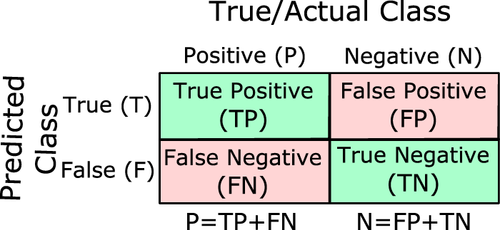
Here the total number of positives and negatives are \(P = TP + FN\) and \(N = TN + FP\), with positives being the minority class. Let the class prevalence be \(\pi = \frac{P}{P + N}\).
A predictor produces a score (probability, log-odds, margin, etc.). A decision rule is a threshold applied to that score, which produces a binary classifier whose outputs are analyzed according to the confusion matrix above. To help choose the decision threshold, the main tools are diagnostic curves like ROC or precision-recall curves. Here we show a few practical tips to using these to assess a predictor.
Content moderation is a widely relevant, real‑world use case where positives are rare (and also skewed across subtypes).
Moderation / safety pipelines (platform comments, forums, issue trackers) use these exact labels and class distributions; the rarest labels (e.g., threat) are the hardest and most critical. The Hugging Face civil_comments dataset is an openly available replica of Jigsaw’s Unintended Bias challenge, and a good .
Strong third-party baselines exist (e.g., Detoxify, MiniLMv2-toxic-jigsaw), making comparisons credible and easy to reproduce. We use the Civil Comments dataset (an open replica of Jigsaw’s Unintended Bias challenge) and compare:
Third‑party pretrained: Detoxify (original/unbiased) out‑of‑the‑box
We report AUPRC (average precision), ROC‑AUC, F1@optimal threshold, and show reliability (ECE) and per‑label PR curves.
# If needed:
# !pip -q install datasets transformers torch torchvision torchaudio scikit-learn --upgrade
# !pip -q install detoxify==0.5.2
# !pip -q install matplotlibThe Civil Comments dataset on Hugging Face has continuous labels in [0,1] (fraction of human annotators). We binarize with thresholds (default 0.5) and keep six main labels: toxicity, severe_toxicity, obscene, threat, insult, identity_attack.
import os, math, time, random, json, numpy as np, pandas as pd
from datasets import load_dataset
from sklearn.model_selection import train_test_split

SEED=1337
random.seed(SEED); np.random.seed(SEED)

LABELS = ['toxicity','severe_toxicity','obscene','threat','insult','identity_attack']
THRESH = {lbl:0.5 for lbl in LABELS}  # can tune per-label thresholds later

ds = load_dataset('google/civil_comments')
df = pd.DataFrame(ds['test']).dropna()

# # binarize
# for lbl in LABELS:
#     df[lbl] = (df[lbl] >= THRESH[lbl]).astype(int)

# # split
# train_df, temp_df = train_test_split(df, test_size=0.2, random_state=SEED, stratify=df['toxicity'])
# valid_df, test_df = train_test_split(temp_df, test_size=0.5, random_state=SEED, stratify=temp_df['toxicity'])

# len(train_df), len(valid_df), len(test_df), {l:int(df[l].sum()) for l in LABELS}

df| text | toxicity | severe_toxicity | obscene | threat | insult | identity_attack | sexual_explicit | |
|---|---|---|---|---|---|---|---|---|
| 0 | [ Integrity means that you pay your debts.]\n\... | 0.000000 | 0.0 | 0.0 | 0.0 | 0.000000 | 0.000000 | 0.0 |
| 1 | This is malfeasance by the Administrator and t... | 0.100000 | 0.0 | 0.0 | 0.0 | 0.100000 | 0.000000 | 0.0 |
| 2 | @Rmiller101 - Spoken like a true elitist. But ... | 0.300000 | 0.0 | 0.0 | 0.0 | 0.200000 | 0.000000 | 0.0 |
| 3 | Paul: Thank you for your kind words. I do, in... | 0.000000 | 0.0 | 0.0 | 0.0 | 0.000000 | 0.000000 | 0.0 |
| 4 | Sorry you missed high school. Eisenhower sent ... | 0.000000 | 0.0 | 0.0 | 0.0 | 0.000000 | 0.000000 | 0.0 |
| ... | ... | ... | ... | ... | ... | ... | ... | ... |
| 97315 | He should lose his job for promoting mis-infor... | 0.000000 | 0.0 | 0.0 | 0.0 | 0.000000 | 0.000000 | 0.0 |
| 97316 | "Thinning project is meant to lower fire dange... | 0.166667 | 0.0 | 0.0 | 0.0 | 0.166667 | 0.166667 | 0.0 |
| 97317 | I hope you millennials are happy that you put ... | 0.400000 | 0.0 | 0.0 | 0.0 | 0.400000 | 0.100000 | 0.0 |
| 97318 | I'm thinking Kellyanne Conway (a.k.a. The Trum... | 0.000000 | 0.0 | 0.0 | 0.0 | 0.000000 | 0.000000 | 0.0 |
| 97319 | I still can't figure why a pizza in AK cost mo... | 0.000000 | 0.0 | 0.0 | 0.0 | 0.000000 | 0.000000 | 0.0 |
97320 rows × 8 columns
df_sample = df.sample(n=10000, random_state=42)
LABELS = ['toxicity','severe_toxicity','obscene','threat','insult','identity_attack']


from detoxify import Detoxify
tox = Detoxify('unbiased-small')

def score_detox(texts, labels, batch=250):
    itime = time.time()
    out = []
    for i in range(0, len(texts), batch):
        chunk = texts[i:i+batch].tolist()
        pred = tox.predict(chunk)
        print(time.time() - itime, pred)
        arr = np.vstack([pred[l] for l in labels]).T
        out.append(arr)
    return np.vstack(out)

p_detox = score_detox(df_sample['text'], LABELS)#np.save('p_detox.npy', p_detox)
p_detox = np.load('p_detox.npy')
pred_df = pd.DataFrame(p_detox, columns=LABELS)
pred_df| toxicity | severe_toxicity | obscene | threat | insult | identity_attack | |
|---|---|---|---|---|---|---|
| 0 | 0.000484 | 0.000002 | 0.000020 | 0.000019 | 0.000284 | 0.000043 |
| 1 | 0.139522 | 0.000008 | 0.000253 | 0.002380 | 0.068277 | 0.000383 |
| 2 | 0.000282 | 0.000003 | 0.000021 | 0.000024 | 0.000134 | 0.000042 |
| 3 | 0.000288 | 0.000003 | 0.000019 | 0.000019 | 0.000133 | 0.000045 |
| 4 | 0.000579 | 0.000002 | 0.000030 | 0.000025 | 0.000214 | 0.000052 |
| ... | ... | ... | ... | ... | ... | ... |
| 9995 | 0.124552 | 0.000003 | 0.000129 | 0.000122 | 0.085931 | 0.001285 |
| 9996 | 0.000906 | 0.000004 | 0.000023 | 0.000236 | 0.000169 | 0.000137 |
| 9997 | 0.141386 | 0.000028 | 0.178269 | 0.000545 | 0.029212 | 0.001454 |
| 9998 | 0.098980 | 0.000254 | 0.000951 | 0.005035 | 0.012753 | 0.054582 |
| 9999 | 0.000318 | 0.000002 | 0.000019 | 0.000021 | 0.000161 | 0.000044 |
10000 rows × 6 columns
labels_df = df_sample[LABELS]
labels_df| toxicity | severe_toxicity | obscene | threat | insult | identity_attack | |
|---|---|---|---|---|---|---|
| 50202 | 0.000000 | 0.0 | 0.0 | 0.000000 | 0.0 | 0.0 |
| 71059 | 0.000000 | 0.0 | 0.0 | 0.000000 | 0.0 | 0.0 |
| 33631 | 0.000000 | 0.0 | 0.0 | 0.000000 | 0.0 | 0.0 |
| 34817 | 0.000000 | 0.0 | 0.0 | 0.000000 | 0.0 | 0.0 |
| 43041 | 0.000000 | 0.0 | 0.0 | 0.000000 | 0.0 | 0.0 |
| ... | ... | ... | ... | ... | ... | ... |
| 54408 | 0.000000 | 0.0 | 0.0 | 0.000000 | 0.0 | 0.0 |
| 2271 | 0.142857 | 0.0 | 0.0 | 0.142857 | 0.0 | 0.0 |
| 70881 | 0.000000 | 0.0 | 0.0 | 0.000000 | 0.0 | 0.0 |
| 90590 | 0.300000 | 0.0 | 0.0 | 0.100000 | 0.2 | 0.4 |
| 73725 | 0.000000 | 0.0 | 0.0 | 0.000000 | 0.0 | 0.0 |
10000 rows × 6 columns
Let’s look at insult classification. The histogram of prediction scores, which in this case map to probabilities, is very common for imbalanced problems - bimodal with almost all the scores near zero.
import matplotlib.pyplot as plt

plt.hist(pred_df['insult'], bins=100)
plt.show()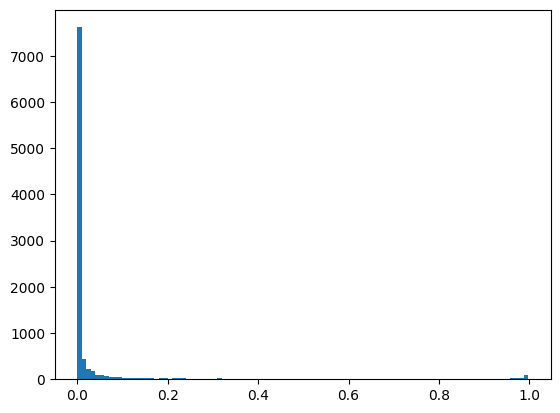
labels_df = (df_sample[LABELS] >= 0.5)
labels_df| toxicity | severe_toxicity | obscene | threat | insult | identity_attack | |
|---|---|---|---|---|---|---|
| 50202 | False | False | False | False | False | False |
| 71059 | False | False | False | False | False | False |
| 33631 | False | False | False | False | False | False |
| 34817 | False | False | False | False | False | False |
| 43041 | False | False | False | False | False | False |
| ... | ... | ... | ... | ... | ... | ... |
| 54408 | False | False | False | False | False | False |
| 2271 | False | False | False | False | False | False |
| 70881 | False | False | False | False | False | False |
| 90590 | False | False | False | False | False | False |
| 73725 | False | False | False | False | False | False |
10000 rows × 6 columns
The ROC curve (Fawcett 2006) measures the tradeoff between true positive rate and false positive rate, defined as:
\[ TPR = \frac{TP}{TP + FN} \qquad FPR = \frac{FP}{FP + TN}\]
When positives are rare, the empirical ROC often looks almost perfect even for mediocre models. There are typically a large fraction of low-scoring negative examples; since all (positive, negative) pairs count the same towards the ROC, these heavily negative examples contribute significantly towards the auROC; small ranking mistakes get “averaged away”, giving deceptively high AUROC scores.
The curve’s shape carries little information in this parametrization. We mostly see a near-vertical left edge, as it is very difficult to achieve high FPR - even the all-negatives predictor achieves low FPR.
We can plot the ROC curve on our imbalanced data and see this also.
Let’s go back to the original problem of evaluating the predictions of the classifier on imbalanced binary data. In practice, a successful classifier should identify many of the positives (high recall). This is easy to achieve by just predicting positive very liberally, so we often want that many of its positive predictions should be correct (high precision). Precision and recall are two of the most common goals for imbalanced classifiers and information retrievers (Saito and Rehmsmeier 2015).
The tradeoff between precision and recall is easy to spot. High recall is achieved by predicting positive liberally, and high precision achieved by predicting positive conservatively. There is no single universally best solution to this tradeoff, so a precision-recall curve is common.
Even for severely imbalanced datasets, it is common to encounter values of precision and recall everywhere from 0 to 1.
So such curves are everywhere for evaluating imbalanced datasets (Davis and Goadrich 2006). Here we overview a few things about them that are practically useful but not widely known.
Precision and recall are defined as \[ p = \frac{TP}{TP + FP} \qquad , \qquad r = \frac{TP}{P} \]
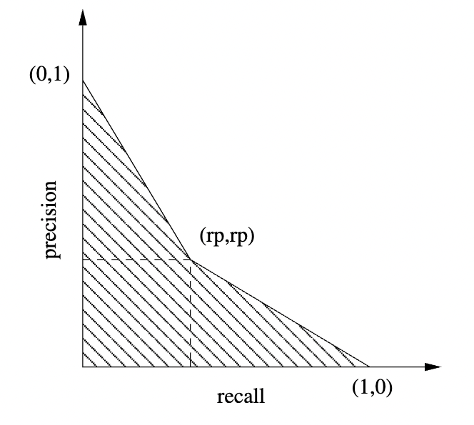
A sample precision-recall curve (PR curve) is easy to plot:
There is actually an “unachievable region” in PR space for any given skew \(\pi\). Because \(FP \leq N−P\), we obtain the Boyd‑Davis lower bound \[ p \geq \frac{\pi r}{1 - \pi + \pi r} \]
We can interpret auPRC as a weighted error, similarly to how we interpreted auROC (McDermott et al. 2024). To quote that paper,
The only difference between AUROC and AUPRC with respect to model dependent parameters… is that optimizing AUROC equates to minimizing the expected false positive rate over all positive samples in an unweighted manner… whereas optimizing AUPRC equates to minimizing the expected false positive rate over all positive samples weighted by the inverse of the model’s “firing rate.”
In other words, as that paper proves, AUPRC prioritizes high-scoring mistakes, instead of treating all mistakes equally.
In practice, auPRC can be notoriously tricky to compute because the PR curve can be irregularly shaped, not convex, and can be quite coarsely-grained along the precision axis. This requires special computational attention to deal with (e.g. (Grau, Grosse, and Keilwagen 2015), (Saito and Rehmsmeier 2017)), which still does not address the key brittleness in trading off precision and recall.
Fortunately, there is a way of surmounting all these issues in a robust manner by thresholding the predictor scores, which we overview next.
There is always a point at which precision and recall are equal.
Setting \(p = r\) in the definitions,
\[ \frac{TP}{P} = \frac{TP}{TP + FP} \implies TP + FP = P \]
Precision equals recall at the threshold that predicts as many positives as actually exist in the data. Equivalently, the predicted positive rate equals the class prevalence \(\pi\).
There will always be such a point for a scoring classifier:
At an extreme high threshold, the first positive that creeps above the cut‑off yields \(p=1>r\).
At a very low threshold, (everything predicted positive) we get \(p=π<r=1\).
Monotone stepping of \(TP+FP\) between those two ends (each new item flagged can only increase that count by 1) ensures at least one crossing of the line \(p=r\), or in discrete terms a pair of adjacent thresholds with \(p \geq r\) and \(p \leq r\).
We will call this the Equilibrium Precision-Recall (EPR) point, but it has been called other names in the past few decades when it has been rediscovered.
Pictorially, we are saying that two things hold:
Any precision-recall curve intersects the line \(y = x\).
At the intersection with \(y = x\), the classifier predicts the same number of positives as actually exist.
This enables us to read off the equilibrium EPR point from any precision-recall curve, like the one we saw earlier.
With this thresholding, all \(F_{\beta}\) values converge to this same equilibrium value, regardless of \(\beta\). It gives robust results; it doesn’t matter how recall and precision are weighed.
This also highlights the importance of knowing the true label prevalence in choosing a robust threshold. It is vital to respect this in case of a distribution shift:
Tune thresholds on a validation set that matches the deployment prevalence; make the predicted prevalence equal to the deployment prevalence to get the EPR threshold.
Average precision, or AUPRC, is notoriously tricky to compute near the edges of the distribution by naive methods, suffering numerical instabilities and more.
Fortunately, there are a few direct ways to deal with this problem, which are useful in many situations:
The equilibrium precision-recall value provides a key intermediate point on the precision-recall curve, between an ultra-conservative threshold with perfect recall and zero precision, and an ultra-aggressive threshold with perfect precision and zero recall.
In practice, many PR curves appear to be piecewise linear at the extremes, subtending triangles under them. The idea then arises (Aslam and Yilmaz 2005) to use these triangles to compute auPRC:
There is a useful one-parameter form for the P-R curve (Aslam and Yilmaz 2005), parametrized by a value \(\alpha \geq -1\),
\[ p (r) = \frac{1 - r}{1 + \alpha r} \]
When we want it to pass through a particular point \((r_0, p_0)\), this gives enough information to determine \(\alpha = \frac{1 - p_0 - r_0}{ p_0 r_0 }\).
In this case, we’re particularly interested in \(p_0 = r_0\), which gives the EPR point. This gives \(\alpha = \frac{1 - 2 p_0 }{ p_0^2 } = \left( (1 / p_0 ) - 1 \right)^2 - 1\).
In addition to passing through the same points as the piecewise linear curve, the domain and range of this curve are automatically [0, 1] as we would like. The curve is also symmetric around the line \(y = x\), to avoid reflecting any inherent bias towards sensitivity or specificity.
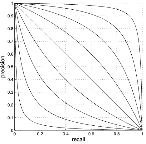
The equilibrium precision-recall point of each curve is where it intersects the line \(y = x\). We can see that for this family of curves, it represents a particularly symmetric intermediate point to fit the model and discriminate between \(\alpha\) values.
The auPRC can be derived analytically from this model. We can calculate the auPRC up to any recall \(r_2 \leq 1\):
\[ AP \approx \frac{(1 + \alpha) \ln (1 + \alpha r_2) - \alpha r_2}{\alpha^2} \]
When \(\alpha = 0\), \(AP \approx r_2 (1 - \frac{1}{2} r_2)\).
Example: if \(r_p = 0.32\), then \(\alpha ≈ 8.8\); at recall 0.8, the model predicts \(p ≈ 0.024\), giving a quick sanity check on how sharply precision will fall for any given recall level.
These minimalist closed‑form curves are rarely documented in standard ML libraries, but they are well‑established in the IR and diagnostic‑testing literature and can be implemented in a few lines once we know which parameter to solve for.
We devise a way to visualize the predictions of classifiers in imbalanced settings. For such visualizations, the main challenge is to use the screen pixels to display relevant information – the true positives – when it is so rare in the data.
Not only are these positives are few and far between, they are also distributed very nonuniformly, largely present towards the top of the model score distribution. We can therefore visualize them by stratifying the positives according to their model score.
For highly imbalanced classification problems, this is a hugely significant change in normalization, which has dramatic results. Let’s illustrate on this data.
We define some style files and colors first. This app works with assets/ files load_screen.css and master_styles.css.
import base64, io, json, argparse, numpy as np, pandas as pd
from sklearn.metrics import roc_auc_score, average_precision_score, precision_recall_curve
PARAMS={'bg_color':'#111111','font_color':'#DDDDDD','legend_font_color':'#CCCCCC','legend_font_size':12,'marker_opacity':0.85}
_color_pos='#3333FF'; _color_amb='#FF0000'; _color_neg='#FFCC00'; _color_hl_pos='#72A7FB'; _color_hl_amb='#A59ABC'; _color_hl_neg='#A5CEBC'; _color_hl='#87CEFA'
legend_font_macro = {
    'family': 'sans-serif', 'size': PARAMS['legend_font_size'], 'color': PARAMS['legend_font_color']}


def parse_dataframe(df):
    df = df.copy()
    cand = [('y_true','y_score'),('label','score'),('labels','preds'),('true','pred')]
    cols = {c.lower():c for c in df.columns}
    use = None
    for a,b in cand:
        if a in cols and b in cols:
            use = (cols[a],cols[b]); break
    if use is None and df.shape[1] >= 2:
        use = (df.columns[0],df.columns[1])
    y_true = np.asarray(df[use[0]]).astype(float)
    y_score = np.asarray(df[use[1]]).astype(float)
    return y_true, y_score


def parse_upload(contents, filename):
    ctype, cstring = contents.split(',')
    decoded = base64.b64decode(cstring)
    if filename.lower().endswith('.json'):
        return parse_dataframe(pd.read_json(io.BytesIO(decoded)))
    if filename.lower().endswith('.npy'):
        D = np.load(io.BytesIO(decoded), allow_pickle=True).item()
        return np.asarray(D['y_true']).astype(float), np.asarray(D['y_score']).astype(float)
    try:
        return parse_dataframe(pd.read_csv(io.BytesIO(decoded)))
    except Exception:
return parse_dataframe(pd.read_csv(io.BytesIO(decoded),sep='\t'))There is a bunch of utility code here that we need in stratifying the data along the prediction scores.
def discrete_deriv(a):
    return (a - np.concatenate(([0], a[:-1])))


def recall_binned_summary(labels_arr, preds_arr, posperbin):
    ranks = np.argsort(preds_arr)[::-1]
    lb = labels_arr[ranks]
    numpos = int(np.sum(lb == 1))
    posperbin = max(1,int(posperbin))
    posperbin = min(posperbin,max(1,numpos))
    edges = np.arange(0,numpos,posperbin)
    cdf_pos = np.cumsum(lb == 1)
    cdf_neg = np.cumsum(lb == 0)
    cdf_amb = np.cumsum(lb == -1)
    left = np.isin(cdf_pos, edges).astype(int)
    bins = np.where(discrete_deriv(left) == 1)[0]
    bins = np.concatenate((bins,[len(left)-1]))
    fpos = discrete_deriv(cdf_pos[bins])
    fneg = discrete_deriv(cdf_neg[bins])
    famb = discrete_deriv(cdf_amb[bins])
    return bins, fpos, fneg, famb
Some more boilerplate code is needed to plot the standard ROC and PRC curves and display the confusion matrix.
def calc_curve(fpos,fneg,mode='prc'):
    denom = np.cumsum(fpos+fneg)
    denom = np.where(denom == 0, 1, denom)
    recalls = np.cumsum(fpos)*(1.0/np.sum(fpos)) if np.sum(fpos)>0 else np.zeros_like(fpos,dtype=float)
    if mode == 'prc':
        return (recalls, np.cumsum(fpos)/denom)
    if mode == 'roc':
        fprs = np.cumsum(fneg)*(1.0/np.sum(fneg)) if np.sum(fneg)>0 else np.zeros_like(fneg,dtype=float)
        return (fprs, recalls)
    if mode == 'confusion':
        tp = np.cumsum(fpos)
        fn = np.sum(fpos) - tp
        fp = np.cumsum(fneg)
        tn = np.sum(fneg) - fp;
        return (tp,fp,fn,tn)


def prepare_stats(y_true, y_score, posperbin):
    y_true = np.asarray(y_true).astype(float); y_score=np.asarray(y_score).astype(float)
    y_true = np.where(np.isin(y_true,[-1,0,1]), y_true, np.where(y_true > 0, 1, 0))
    bins, fpos, fneg, famb = recall_binned_summary(y_true, y_score, posperbin)
    st = {'bins_edges':bins, 'bin_freqs_pos':fpos, 'bin_freqs_neg':fneg, 'bin_freqs_amb':famb}
    st['bin_freqs'] = fpos+fneg+famb
    st['prc'] = calc_curve(fpos,fneg,'prc')
    st['roc'] = calc_curve(fpos,fneg,'roc')
    st['confusion'] = calc_curve(fpos,fneg,'confusion')
    ranks = np.argsort(y_score)[::-1]
    cum = np.cumsum(st['bin_freqs'])-1
    cum = np.clip(cum,0,len(ranks)-1)
    st['thresh_as_pred'] = y_score[ranks[cum]]
    st['beta'] = np.sum(fneg)/max(1,np.sum(fpos))
    st['auroc'] = float(roc_auc_score(np.where(y_true>=0,y_true,0), y_score))
    prec,rec,_ = precision_recall_curve(np.where(y_true==1,1,0), y_score)
    st['auprc'] = float(average_precision_score(np.where(y_true==1,1,0), y_score))
    return st
Finally, it is useful to wrap some of the visualization code, which produces Plotly interactive panels given the data.
def build_prc_figure(st, slider_val):
    rec,prec=st['prc']; n=max(1,len(st['bin_freqs_pos'])); idx=round(slider_val*n)-1
    cx=0.0 if idx<0 else rec[idx]; cy=1.0 if idx<0 else prec[idx]
    return {'data':[{'name':'Precision-recall','x':rec,'y':prec,'fill':'tozeroy','mode':'lines','type':'scatter'},
                    {'name':'Classifier','x':[cx],'y':[cy],'mode':'markers','marker':{'size':10,'symbol':'circle','color':_color_hl,'line':{'color':'white','width':1}},'type':'scatter'}],
            'layout':{'showlegend':False,'title':'Precision–Recall','titlefont':{'family':'sans-serif','color':PARAMS['legend_font_color'],'size':20},
                      'clickmode':'event+select','hovermode':'closest','uirevision':'default',
                      'xaxis':{'title':'Recall','titlefont':legend_font_macro,'automargin':True,'showticklabels':True,'tickfont':legend_font_macro},
                      'yaxis':{'title':'Precision','titlefont':legend_font_macro,'showticklabels':True,'tickfont':legend_font_macro},
                      'plot_bgcolor':PARAMS['bg_color'],'paper_bgcolor':PARAMS['bg_color']}}


def build_roc_figure(st, slider_val):
    fpr,tpr = st['roc']
    n = max(1,len(st['bin_freqs_pos']))
    idx = round(slider_val*n)-1
    cx = 0.0 if idx<0 else fpr[idx]
    cy = 1.0 if idx<0 else tpr[idx]
    return {'data':[{'name':'ROC curve','x':fpr,'y':tpr,'fill':'tozeroy','mode':'lines','type':'scatter'},
                    {'name':'Classifier','x':[cx],'y':[cy],'mode':'markers','marker':{'size':10,'symbol':'circle','color':_color_hl,'line':{'color':'white','width':1}},'type':'scatter'}],
            'layout':{'showlegend':False,'title':'ROC','titlefont':{'family':'sans-serif','color':PARAMS['legend_font_color'],'size':20},
                      'clickmode':'event+select','hovermode':'closest','uirevision':'default',
                      'xaxis':{'title':'FPR','titlefont':legend_font_macro,'automargin':True,'showticklabels':True,'tickfont':legend_font_macro},
                      'yaxis':{'title':'TPR','titlefont':legend_font_macro,'showticklabels':True,'tickfont':legend_font_macro},
                      'plot_bgcolor':PARAMS['bg_color'],'paper_bgcolor':PARAMS['bg_color']}}


def build_confusion_text(st, slider_val):
    n=max(1,len(st['bin_freqs_pos'])); idx=round(slider_val*n)-1
    if idx<0:
        tp = 0
        fp = 0
        fn = int(np.sum(st['bin_freqs_pos']))
        tn = int(np.sum(st['bin_freqs_neg']))
        r = 0.0; p = 1.0; fpr = 0.0
    else:
        tp = int(st['confusion'][0][idx])
        fp = int(st['confusion'][1][idx])
        fn = int(st['confusion'][2][idx])
        tn = int(st['confusion'][3][idx])
        r = st['prc'][0][idx]; p=st['prc'][1][idx]; fpr=st['roc'][0][idx]
    return {
        'tp':tp, 'fp':fp, 'fn':fn, 'tn':tn,
        'recall':float(r), 'precision':float(p), 'fpr':float(fpr)
    }


def build_bars_figure(st, slider_val, mode='relative'):
    bins = st['bins_edges']
    fpos = np.array(st['bin_freqs_pos']); famb = np.array(st['bin_freqs_amb']); fneg = np.array(st['bin_freqs_neg'])
    freq = st['bin_freqs']
    if mode == 'relative':
        fpos = np.divide(fpos, np.where(freq == 0, 1, freq))
        famb = np.divide(famb, np.where(freq == 0, 1, freq))
        fneg = np.divide(fneg, np.where(freq == 0, 1, freq))
        sep_max = 1.0
        y_title = 'Relative frequency'
    else:
        fpos = np.log2(1+fpos); famb=np.log2(1+famb); fneg=np.log2(1+fneg)
        sep_max = float(np.max(fneg)+np.max(famb)+np.max(fpos))
        y_title = 'log2 (1 + count)'
    absc = np.arange(len(bins))/max(1,len(bins)); xthr=float(slider_val)
    shapes = [{'type':'line','xref':'x','yref':'y','line':{'color':_color_hl,'width':5},'x0':xthr,'y0':-0.05,'x1':xthr,'y1':sep_max*1.05},
            {'type':'rect','xref':'x','yref':'y','x0':0,'y0':0,'x1':xthr,'y1':sep_max,'fillcolor':_color_hl,'opacity':0.25,'line':{'width':0}}]
    data = [{'name':'Positives','x':absc,'y':fpos,'marker':{'color':_color_pos},'type':'bar','hoverinfo':'y'},
          {'name':'Ambiguous','x':absc,'y':famb,'marker':{'color':_color_amb},'type':'bar','hoverinfo':'y'},
          {'name':'Negatives','x':absc,'y':fneg,'marker':{'color':_color_neg},'type':'bar','hoverinfo':'y'}]
    return {'data':data,'layout':{'barmode':'stack','margin':{'l':0,'r':0,'b':0,'t':5},'hovermode':'closest','uirevision':'default',
            'xaxis':{'showticklabels':True,'title':{'text':'Recall','font':legend_font_macro},'range':[0,1]},
            'yaxis':{'title':{'text':y_title,'font':legend_font_macro},'showticklabels':False,'showgrid':False,'showline':False,'zeroline':False},
'shapes':shapes,'legend':{'y':'1.1','font':legend_font_macro,'orientation':'h'},'plot_bgcolor':PARAMS['bg_color'],'paper_bgcolor':PARAMS['bg_color']}}With these tools, we create a interactive dashboard, which is a Dash object app. The object is an HTML-style nested one, containing a full-style specification of the entire interface.
def create_app(y_true_default, y_score_default, posperbin_default=3):
    numpos = (y_true_default == 1).sum()
    threshold_default = np.sort(y_score_default)[::-1][numpos]
    import dash
    from dash import dcc, html
    from dash.dependencies import Input, Output, State
    style_text={'textAlign':'center','width':'100%','border':'thin lightgrey solid','color':PARAMS['font_color']}
    app=dash.Dash(__name__); server=app.server
    app.layout=html.Div(className='container',children=[
        html.Div(className='row',children=[
            html.H1('Imbalanced binary predictor evaluation',style={'textAlign':'center','width':'100%','color':PARAMS['font_color']})
        ]),
        html.Div(className='row',children=[
            html.Div(className='three columns',children=[dcc.Upload(id='upload-data',children=html.Div([html.P('Upload CSV',id='upload-button',style=style_text)]) )]),
            html.Div(className='three columns',children=[html.Div(children=[
                html.P('Positives per bin',style={'textAlign':'center','width':'100%','color':PARAMS['font_color']}),
                dcc.Input(id='posperbin',type='number',value=posperbin_default,min=1,step=1,style={'textAlign':'center','width':'100%'})
            ])]),
            html.Div(className='three columns',children=[dcc.RadioItems(id='mode-relative',options=[{'label':'Absolute','value':'absolute'},{'label':'Relative','value':'relative'}],value='relative',style=legend_font_macro,labelStyle={'margin-right':'5px'})]),
            html.Div(className='three columns',children=[html.Div(id='dataset-stats',style={'color':PARAMS['font_color']})])
        ]),
        html.Div(className='row',children=[
            html.Div(className='eight columns',children=[dcc.Graph(id='main-plot',config={'displaylogo':False,'displayModeBar':True},style={'height':'40vh','padding-bottom':'10px'}),
                                                        dcc.Slider(id='slider-pred-threshold',min=0,max=1,step=0.01,value=threshold_default,marks=None,tooltip={"placement": "bottom", "always_visible": True}),
                                                        html.Div(id='confusion-matrix',style={'padding-top':'7px'})],style={'padding-bottom':'15px'}),
            html.Div(className='four columns',children=[dcc.Graph(id='prc-plot',config={'displaylogo':False,'displayModeBar':True},style={'height':'40vh','padding-top':'10px'}),
                                                        dcc.Graph(id='roc-plot',config={'displaylogo':False,'displayModeBar':True},style={'height':'40vh','padding-top':'10px'})],style={'padding-bottom':'15px'})
        ]),
        dcc.Store(id='stored-stats',data=None),
        dcc.Store(id='stored-raw',data=None)
    ],
    style={'width':'100vw','max-width':'none'})

    @app.callback(Output('stored-raw','data'),Input('upload-data','contents'),State('upload-data','filename'))
    def _load(contents,filename):
        if not contents: return None
        y_true,y_score=parse_upload(contents,filename)
        return {'y_true':y_true.tolist(),'y_score':y_score.tolist()}

    @app.callback(Output('stored-stats','data'),[Input('stored-raw','data'),Input('posperbin','value')])
    def _stats(raw,posperbin):
        if raw is None:
            y_true = y_true_default
            y_score = y_score_default
        else:
            y_true = np.asarray(raw['y_true'])
            y_score = np.asarray(raw['y_score'])
        st = prepare_stats(y_true, y_score, posperbin)
        return {k:(v.tolist() if isinstance(v,np.ndarray) else v) for k,v in st.items()}

    @app.callback(Output('dataset-stats','children'),Input('stored-stats','data'))
    def _dsinfo(st):
        if not st: return ''
        pos = int(np.sum(st['bin_freqs_pos']))
        neg = int(np.sum(st['bin_freqs_neg']))
        amb = int(np.sum(st['bin_freqs_amb']))
        beta = st['beta']
        return f"Pos: {pos} | Neg: {neg} | Amb: {amb} | β={beta:.2f} | auPRC={st['auprc']:.3f} | auROC={st['auroc']:.3f}"

    @app.callback(Output('slider-pred-threshold','step'),Input('stored-stats','data'))
    def _slider_step(st): return round(1.0/max(1,len(st['bin_freqs_pos'])), 2) if st else 0.01

    @app.callback(Output('prc-plot','figure'),[Input('stored-stats','data'),Input('slider-pred-threshold','value')])
    def _prc(st,val):
        return build_prc_figure({k:(np.array(v) if isinstance(v,list) else v) for k,v in st.items()}, val or 0.5) if st else {'data':[],'layout':{}}

    @app.callback(Output('roc-plot','figure'),[Input('stored-stats','data'),Input('slider-pred-threshold','value')])
    def _roc(st,val):
        return build_roc_figure({k:(np.array(v) if isinstance(v,list) else v) for k,v in st.items()}, val or 0.5) if st else {'data':[],'layout':{}}

    @app.callback(Output('confusion-matrix','children'),[Input('stored-stats','data'),Input('slider-pred-threshold','value')])
    def _confusion_matrix(st,val):
        if not st: return ''
        st2 = {k:(np.array(v) if isinstance(v,list) else v) for k,v in st.items()}
        o = build_confusion_text(st2,val or 0.5); from dash import html; sty = {'textAlign':'center','width':'100%','color':PARAMS['font_color']}
        return [
            html.P(f"TP: {o['tp']}",style=sty),
            html.P(f"FP: {o['fp']}",style=sty),
            html.P(f"FN: {o['fn']}",style=sty),
            html.P(f"TN: {o['tn']}",style=sty),
            html.P(f"Recall: {o['recall']:.3f}",style=sty),
            html.P(f"Precision: {o['precision']:.3f}",style=sty),
            html.P(f"FPR: {o['fpr']:.3f}",style=sty)]

    @app.callback(Output('main-plot','figure'),[Input('stored-stats','data'),Input('slider-pred-threshold','value'),Input('mode-relative','value')])
    def _bars(st,val,mode):
        return build_bars_figure({k:(np.array(v) if isinstance(v,list) else v) for k,v in st.items()}, val or 0.5, mode or 'relative') if st else {'data':[],'layout':{}}
return app,serverall_code = r'''import base64, io, json, argparse, numpy as np, pandas as pd
from sklearn.metrics import roc_auc_score, average_precision_score, precision_recall_curve
PARAMS={'bg_color':'#111111','font_color':'#DDDDDD','legend_font_color':'#CCCCCC','legend_font_size':12,'marker_opacity':0.85}
_color_pos='#3333FF'; _color_amb='#FF0000'; _color_neg='#FFCC00'; _color_hl_pos='#72A7FB'; _color_hl_amb='#A59ABC'; _color_hl_neg='#A5CEBC'; _color_hl='#87CEFA'
legend_font_macro = {
'family': 'sans-serif', 'size': PARAMS['legend_font_size'], 'color': PARAMS['legend_font_color']}
def discrete_deriv(a):
return (a - np.concatenate(([0], a[:-1])))
def parse_dataframe(df):
df = df.copy()
cand = [('y_true','y_score'),('label','score'),('labels','preds'),('true','pred')]
cols = {c.lower():c for c in df.columns}
use = None
for a,b in cand:
if a in cols and b in cols:
use = (cols[a],cols[b]); break
if use is None and df.shape[1] >= 2:
use = (df.columns[0],df.columns[1])
y_true = np.asarray(df[use[0]]).astype(float)
y_score = np.asarray(df[use[1]]).astype(float)
return y_true, y_score
def parse_upload(contents, filename):
ctype, cstring = contents.split(',')
decoded = base64.b64decode(cstring)
if filename.lower().endswith('.json'):
return parse_dataframe(pd.read_json(io.BytesIO(decoded)))
if filename.lower().endswith('.npy'):
D = np.load(io.BytesIO(decoded), allow_pickle=True).item()
return np.asarray(D['y_true']).astype(float), np.asarray(D['y_score']).astype(float)
try:
return parse_dataframe(pd.read_csv(io.BytesIO(decoded)))
except Exception:
return parse_dataframe(pd.read_csv(io.BytesIO(decoded),sep='\t'))
def recall_binned_summary(labels_arr, preds_arr, posperbin):
ranks = np.argsort(preds_arr)[::-1]
lb = labels_arr[ranks]
numpos = int(np.sum(lb == 1))
posperbin = max(1,int(posperbin))
posperbin = min(posperbin,max(1,numpos))
edges = np.arange(0,numpos,posperbin)
cdf_pos = np.cumsum(lb == 1)
cdf_neg = np.cumsum(lb == 0)
cdf_amb = np.cumsum(lb == -1)
left = np.isin(cdf_pos, edges).astype(int)
bins = np.where(discrete_deriv(left) == 1)[0]
bins = np.concatenate((bins,[len(left)-1]))
fpos = discrete_deriv(cdf_pos[bins])
fneg = discrete_deriv(cdf_neg[bins])
famb = discrete_deriv(cdf_amb[bins])
return bins, fpos, fneg, famb
def calc_curve(fpos,fneg,mode='prc'):
denom = np.cumsum(fpos+fneg)
denom = np.where(denom == 0, 1, denom)
recalls = np.cumsum(fpos)*(1.0/np.sum(fpos)) if np.sum(fpos)>0 else np.zeros_like(fpos,dtype=float)
if mode == 'prc':
return (recalls, np.cumsum(fpos)/denom)
if mode == 'roc':
fprs = np.cumsum(fneg)*(1.0/np.sum(fneg)) if np.sum(fneg)>0 else np.zeros_like(fneg,dtype=float)
return (fprs, recalls)
if mode == 'confusion':
tp = np.cumsum(fpos)
fn = np.sum(fpos) - tp
fp = np.cumsum(fneg)
tn = np.sum(fneg) - fp;
return (tp,fp,fn,tn)
def prepare_stats(y_true, y_score, posperbin):
y_true = np.asarray(y_true).astype(float); y_score=np.asarray(y_score).astype(float)
y_true = np.where(np.isin(y_true,[-1,0,1]), y_true, np.where(y_true > 0, 1, 0))
bins, fpos, fneg, famb = recall_binned_summary(y_true, y_score, posperbin)
st = {'bins_edges':bins, 'bin_freqs_pos':fpos, 'bin_freqs_neg':fneg, 'bin_freqs_amb':famb}
st['bin_freqs'] = fpos+fneg+famb
st['prc'] = calc_curve(fpos,fneg,'prc')
st['roc'] = calc_curve(fpos,fneg,'roc')
st['confusion'] = calc_curve(fpos,fneg,'confusion')
ranks = np.argsort(y_score)[::-1]
cum = np.cumsum(st['bin_freqs'])-1
cum = np.clip(cum,0,len(ranks)-1)
st['thresh_as_pred'] = y_score[ranks[cum]]
st['beta'] = np.sum(fneg)/max(1,np.sum(fpos))
st['auroc'] = float(roc_auc_score(np.where(y_true>=0,y_true,0), y_score))
prec,rec,_ = precision_recall_curve(np.where(y_true==1,1,0), y_score)
st['auprc'] = float(average_precision_score(np.where(y_true==1,1,0), y_score))
return st
def build_prc_figure(st, slider_val):
rec,prec=st['prc']; n=max(1,len(st['bin_freqs_pos'])); idx=round(slider_val*n)-1
cx=0.0 if idx<0 else rec[idx]; cy=1.0 if idx<0 else prec[idx]
return {'data':[{'name':'Precision-recall','x':rec,'y':prec,'fill':'tozeroy','mode':'lines','type':'scatter'},
{'name':'Classifier','x':[cx],'y':[cy],'mode':'markers','marker':{'size':10,'symbol':'circle','color':_color_hl,'line':{'color':'white','width':1}},'type':'scatter'}],
'layout':{'showlegend':False,'title':'Precision–Recall','titlefont':{'family':'sans-serif','color':PARAMS['legend_font_color'],'size':20},
'clickmode':'event+select','hovermode':'closest','uirevision':'default',
'xaxis':{'title':'Recall','titlefont':legend_font_macro,'automargin':True,'showticklabels':True,'tickfont':legend_font_macro},
'yaxis':{'title':'Precision','titlefont':legend_font_macro,'showticklabels':True,'tickfont':legend_font_macro},
'plot_bgcolor':PARAMS['bg_color'],'paper_bgcolor':PARAMS['bg_color']}}
def build_roc_figure(st, slider_val):
fpr,tpr = st['roc']
n = max(1,len(st['bin_freqs_pos']))
idx = round(slider_val*n)-1
cx = 0.0 if idx<0 else fpr[idx]
cy = 1.0 if idx<0 else tpr[idx]
return {'data':[{'name':'ROC curve','x':fpr,'y':tpr,'fill':'tozeroy','mode':'lines','type':'scatter'},
{'name':'Classifier','x':[cx],'y':[cy],'mode':'markers','marker':{'size':10,'symbol':'circle','color':_color_hl,'line':{'color':'white','width':1}},'type':'scatter'}],
'layout':{'showlegend':False,'title':'ROC','titlefont':{'family':'sans-serif','color':PARAMS['legend_font_color'],'size':20},
'clickmode':'event+select','hovermode':'closest','uirevision':'default',
'xaxis':{'title':'FPR','titlefont':legend_font_macro,'automargin':True,'showticklabels':True,'tickfont':legend_font_macro},
'yaxis':{'title':'TPR','titlefont':legend_font_macro,'showticklabels':True,'tickfont':legend_font_macro},
'plot_bgcolor':PARAMS['bg_color'],'paper_bgcolor':PARAMS['bg_color']}}
def build_confusion_text(st, slider_val):
n=max(1,len(st['bin_freqs_pos'])); idx=round(slider_val*n)-1
if idx<0:
tp = 0
fp = 0
fn = int(np.sum(st['bin_freqs_pos']))
tn = int(np.sum(st['bin_freqs_neg']))
r = 0.0; p = 1.0; fpr = 0.0
else:
tp = int(st['confusion'][0][idx])
fp = int(st['confusion'][1][idx])
fn = int(st['confusion'][2][idx])
tn = int(st['confusion'][3][idx])
r = st['prc'][0][idx]; p=st['prc'][1][idx]; fpr=st['roc'][0][idx]
return {
'tp':tp, 'fp':fp, 'fn':fn, 'tn':tn,
'recall':float(r), 'precision':float(p), 'fpr':float(fpr)
}
def build_bars_figure(st, slider_val, mode='relative'):
bins = st['bins_edges']
fpos = np.array(st['bin_freqs_pos']); famb = np.array(st['bin_freqs_amb']); fneg = np.array(st['bin_freqs_neg'])
freq = st['bin_freqs']
if mode == 'relative':
fpos = np.divide(fpos, np.where(freq == 0, 1, freq))
famb = np.divide(famb, np.where(freq == 0, 1, freq))
fneg = np.divide(fneg, np.where(freq == 0, 1, freq))
sep_max = 1.0
y_title = 'Relative frequency'
else:
fpos = np.log2(1+fpos); famb=np.log2(1+famb); fneg=np.log2(1+fneg)
sep_max = float(np.max(fneg)+np.max(famb)+np.max(fpos))
y_title = 'log2 (1 + count)'
absc = np.arange(len(bins))/max(1,len(bins)); xthr=float(slider_val)
shapes = [{'type':'line','xref':'x','yref':'y','line':{'color':_color_hl,'width':5},'x0':xthr,'y0':-0.05,'x1':xthr,'y1':sep_max*1.05},
{'type':'rect','xref':'x','yref':'y','x0':0,'y0':0,'x1':xthr,'y1':sep_max,'fillcolor':_color_hl,'opacity':0.25,'line':{'width':0}}]
data = [{'name':'Positives','x':absc,'y':fpos,'marker':{'color':_color_pos},'type':'bar','hoverinfo':'y'},
{'name':'Ambiguous','x':absc,'y':famb,'marker':{'color':_color_amb},'type':'bar','hoverinfo':'y'},
{'name':'Negatives','x':absc,'y':fneg,'marker':{'color':_color_neg},'type':'bar','hoverinfo':'y'}]
return {'data':data,'layout':{'barmode':'stack','margin':{'l':0,'r':0,'b':0,'t':5},'hovermode':'closest','uirevision':'default',
'xaxis':{'showticklabels':True,'title':{'text':'Recall','font':legend_font_macro},'range':[0,1]},
'yaxis':{'title':{'text':y_title,'font':legend_font_macro},'showticklabels':False,'showgrid':False,'showline':False,'zeroline':False},
'shapes':shapes,'legend':{'y':'1.1','font':legend_font_macro,'orientation':'h'},'plot_bgcolor':PARAMS['bg_color'],'paper_bgcolor':PARAMS['bg_color']}}
def create_app(y_true_default, y_score_default, posperbin_default=3):
numpos = (y_true_default == 1).sum()
threshold_default = np.sort(y_score_default)[::-1][numpos]
import dash
from dash import dcc, html
from dash.dependencies import Input, Output, State
style_text={'textAlign':'center','width':'100%','border':'thin lightgrey solid','color':PARAMS['font_color']}
app=dash.Dash(__name__); server=app.server
app.layout=html.Div(className='container',children=[
html.Div(className='row',children=[
html.H1('Imbalanced binary predictor evaluation',style={'textAlign':'center','width':'100%','color':PARAMS['font_color']})
]),
html.Div(className='row',children=[
html.Div(className='three columns',children=[dcc.Upload(id='upload-data',children=html.Div([html.P('Upload CSV',id='upload-button',style=style_text)]) )]),
html.Div(className='three columns',children=[html.Div(children=[
html.P('Positives per bin',style={'textAlign':'center','width':'100%','color':PARAMS['font_color']}),
dcc.Input(id='posperbin',type='number',value=posperbin_default,min=1,step=1,style={'textAlign':'center','width':'100%'})
])]),
html.Div(className='three columns',children=[dcc.RadioItems(id='mode-relative',options=[{'label':'Absolute','value':'absolute'},{'label':'Relative','value':'relative'}],value='relative',style=legend_font_macro,labelStyle={'margin-right':'5px'})]),
html.Div(className='three columns',children=[html.Div(id='dataset-stats',style={'color':PARAMS['font_color']})])
]),
html.Div(className='row',children=[
html.Div(className='eight columns',children=[dcc.Graph(id='main-plot',config={'displaylogo':False,'displayModeBar':True},style={'height':'40vh','padding-bottom':'10px'}),
dcc.Slider(id='slider-pred-threshold',min=0,max=1,step=0.01,value=threshold_default,marks=None,tooltip={"placement": "bottom", "always_visible": True}),
html.Div(id='confusion-matrix',style={'padding-top':'7px'})],style={'padding-bottom':'15px'}),
html.Div(className='four columns',children=[dcc.Graph(id='prc-plot',config={'displaylogo':False,'displayModeBar':True},style={'height':'40vh','padding-top':'10px'}),
dcc.Graph(id='roc-plot',config={'displaylogo':False,'displayModeBar':True},style={'height':'40vh','padding-top':'10px'})],style={'padding-bottom':'15px'})
]),
dcc.Store(id='stored-stats',data=None),
dcc.Store(id='stored-raw',data=None)
],
style={'width':'100vw','max-width':'none'})
@app.callback(Output('stored-raw','data'),Input('upload-data','contents'),State('upload-data','filename'))
def _load(contents,filename):
if not contents: return None
y_true,y_score=parse_upload(contents,filename)
return {'y_true':y_true.tolist(),'y_score':y_score.tolist()}
@app.callback(Output('stored-stats','data'),[Input('stored-raw','data'),Input('posperbin','value')])
def _stats(raw,posperbin):
if raw is None:
y_true = y_true_default
y_score = y_score_default
else:
y_true = np.asarray(raw['y_true'])
y_score = np.asarray(raw['y_score'])
st = prepare_stats(y_true, y_score, posperbin)
return {k:(v.tolist() if isinstance(v,np.ndarray) else v) for k,v in st.items()}
@app.callback(Output('dataset-stats','children'),Input('stored-stats','data'))
def _dsinfo(st):
if not st: return ''
pos = int(np.sum(st['bin_freqs_pos']))
neg = int(np.sum(st['bin_freqs_neg']))
amb = int(np.sum(st['bin_freqs_amb']))
beta = st['beta']
return f"Pos: {pos} | Neg: {neg} | Amb: {amb} | β={beta:.2f} | auPRC={st['auprc']:.3f} | auROC={st['auroc']:.3f}"
@app.callback(Output('slider-pred-threshold','step'),Input('stored-stats','data'))
def _slider_step(st): return round(1.0/max(1,len(st['bin_freqs_pos'])), 2) if st else 0.01
@app.callback(Output('prc-plot','figure'),[Input('stored-stats','data'),Input('slider-pred-threshold','value')])
def _prc(st,val):
return build_prc_figure({k:(np.array(v) if isinstance(v,list) else v) for k,v in st.items()}, val or 0.5) if st else {'data':[],'layout':{}}
@app.callback(Output('roc-plot','figure'),[Input('stored-stats','data'),Input('slider-pred-threshold','value')])
def _roc(st,val):
return build_roc_figure({k:(np.array(v) if isinstance(v,list) else v) for k,v in st.items()}, val or 0.5) if st else {'data':[],'layout':{}}
@app.callback(Output('confusion-matrix','children'),[Input('stored-stats','data'),Input('slider-pred-threshold','value')])
def _confusion_matrix(st,val):
if not st: return ''
st2 = {k:(np.array(v) if isinstance(v,list) else v) for k,v in st.items()}
o = build_confusion_text(st2,val or 0.5); from dash import html; sty = {'textAlign':'center','width':'100%','color':PARAMS['font_color']}
return [
html.P(f"TP: {o['tp']}",style=sty),
html.P(f"FP: {o['fp']}",style=sty),
html.P(f"FN: {o['fn']}",style=sty),
html.P(f"TN: {o['tn']}",style=sty),
html.P(f"Recall: {o['recall']:.3f}",style=sty),
html.P(f"Precision: {o['precision']:.3f}",style=sty),
html.P(f"FPR: {o['fpr']:.3f}",style=sty)]
@app.callback(Output('main-plot','figure'),[Input('stored-stats','data'),Input('slider-pred-threshold','value'),Input('mode-relative','value')])
def _bars(st,val,mode):
return build_bars_figure({k:(np.array(v) if isinstance(v,list) else v) for k,v in st.items()}, val or 0.5, mode or 'relative') if st else {'data':[],'layout':{}}
return app,server
'''numpos = (y_true_default == 1).sum()
threshold_default = np.sort(y_score_default)[::-1][numpos]
print(threshold_default, numpos)0.3277915418148041 63file_pfx = "../../files/dashboards/"
with open(file_pfx + "imbalanced_classifiers_dash.py", "w", encoding="utf-8") as f:
f.write(all_code)The only thing left is to load data into this browser and discover what can be seen by stratifying the data by model scores in this way.
For a visualization, we want enough bins to make the stratification meaningful, but not too many because otherwise the real positives would be too finely split. We don’t want more than around 100 bins, regardless of the true number of positives. For low numbers of positives, we just want 2-3 per bin.
decomp_tools_path = "../../files/dashboards/" + "imbalanced_classifiers_dash.py"

from importlib.machinery import SourceFileLoader
imbalanced_classifiers_dash = SourceFileLoader("imbalanced_classifiers_dash", decomp_tools_path).load_module()

# import imbalanced_dash_app, importlib
# importlib.reload(imbalanced_dash_app)


default_label = 'insult'
y_true_default = labels_df[default_label]
y_score_default = pred_df[default_label]

# Set the number of positive examples per bin to be a sensible default
max_num_bins = 100
pos_total = np.sum(y_true_default)
posperbin_default_min = 2
posperbin_default_max = pos_total // max_num_bins
posperbin_default = posperbin_default_max if pos_total > (posperbin_default_min*max_num_bins) else posperbin_default_min

app, _ = imbalanced_classifiers_dash.create_app(y_true_default, y_score_default, posperbin_default=posperbin_default)
app.run(debug=True)
This effectively re-normalizes the x-axis on the histogram of scores, plotting the score distribution (x-axis) vs. the label distribution (y-axis). It makes it easy to visually see which thresholds would lead to which precision and recall, and uses roughly the same amount of screen real estate for each quantile of actual positive signal.
@online{balsubramani,
  author = {Balsubramani, Akshay},
  title = {Evaluating Extremely Imbalanced Classification},
  langid = {en}
}