Multi-criterion optimization and decision-making

The power of weighted sums

Why trade‑offs matter

Real‑world decisions in areas like drug discovery, investment portfolio allocation, and recommender systems rarely optimize a single scalar.
In each of those situations, many partially‑conflicting desiderata must be juggled (efficacy vs. toxicity, return vs. risk, relevance vs. diversity).

When objectives pull in different directions, we ask:

What does “better” even mean when no option is best on all axes?

Multi-objective optimization is notoriously under-determined, for precizely the reason that there are multiple objectives instead of just one. The final decision intuitively depends on how different objectives are weighed in decision-making; considering different objectives as “most important” will lead to different results.

A couple of these intuitions are quite generally true. We’ll emphasize them and continue to quantitatively develop them in this post:

• Weighting. When there are two objectives, the decision problem amounts to setting one relative weight. And in general for \(K\) objectives, it amounts to setting \(K-1\) relative weights. The weights are \(\geq 0\), and indicate the relative “prices” of lowering each of the objectives.

• Normalization. Each objective can, in general, be on a different scale, which complicates the process of finding a good solution and interpreting it. But normalizing the objectives, by replacing each value by its percentile in the data, can help.

This shifts the approach from pure “optimization” to what’s often called “frontier exploration,” referring to the Pareto frontier. It takes another set of heuristics (in the simplest case, just a human judging the various solutions) to decide on the best path forward – how to weigh the objectives. To that point, any method which generates a medium-large quantity of decent solutions will give the decision-maker what is needed.

The important part about these kinds of optimizations is to understand how one’s own implementation explores the configuration space. That has more to do with the understanding of the problem than the specific algorithm that’s used.

Now we formalize the core notions of the Pareto frontier and dominance, and then explore how to reduce these problems to single-objective versions with weighted-sum scalarization and duality.

Choosing among multiple objectives

We have \(K \geq 2\) real‑valued objectives
\[ f_k: \mathcal{X} \to \mathbb{R}, \qquad k=1,\dots,K \] evaluated on alternatives \(x\in\mathcal X\) (suppose these are molecules in a drug discovery program).

We assume larger is better; if an objective should be minimized (e.g. toxicity), negate it. Write the vector of scores as \(f (x) = (f_1 (x), \dots, f_K (x))\).

Pareto dominance

As discussed above, \(x\) is typically not directly comparable to \(y\) in MOO problems, because comparison occurs along \(K\) different axes. But there are many potential molecules which are not good in any criterion,

\(x\) dominates \(y\) (\(x\succ y\)) iff
\[ \forall k : \; f_k (x) \geq f_k (y) \quad \text{and} \quad \exists k : \; f_k (x) > f_k (y). \]

The Pareto set
\[ \mathcal{P} = \{ x \in \mathcal{X} : \nexists y \in \mathcal{X} \text{ s.t. } y \succ x \} \] collects the undominated options; its image \(f (\mathcal{P})\) is the Pareto front.

A Pareto‑optimal point cannot be improved without hurting at least one criterion. Alternatively, non-Pareto-optimal points can be improved in some way without hurting any of the criteria.

import numpy as np


def pareto_front(points, maximize_array=None):
    """
    Find the Pareto front of a set of points.

    Parameters
    ----------
    points : array-like of shape (n_points, n_criteria)
        A set of points in n-dimensional space.
    maximize_array : array-like of shape (n_criteria,)
        A boolean array indicating which criteria should be maximized.

    Returns
    -------
    is_efficient : array-like of shape (n_points,)
        A boolean array indicating which points are on the Pareto front.
    """
    if maximize_array is None:
        maximize_array = np.ones(points.shape[1], dtype=bool)
    else:
        assert len(maximize_array) == points.shape[1], "maximize_array must be the same length as the number of criteria"
        maximize_array = np.array(maximize_array)
    # flip the signs of points that should be minimized
    points = np.multiply(points, 2 * maximize_array - 1)
    # Initialize all points as efficient
    is_efficient = np.ones(points.shape[0], dtype=bool)
    for i, c in enumerate(points):
        if is_efficient[i]:
            is_efficient[is_efficient] = np.any(points[is_efficient] > c, axis=1)
            is_efficient[i] = True
    return is_efficient

Scalarization by weighting

Because \(\mathcal P\) is typically large or continuous, we need a decision rule to pick a single \(x^\star\).
Common scalarizations turn the \(K\) scores into one number. It turns out that the most common scalarization method, of taking a weighted combination of the multiple objectives, is sufficient to be a general approach for almost any mulltiobjective problem. The reasons why are technical but fundamental. We briefly overview them here.

Constrained optimization

The most straightforward way is probably to pick an anchor objective to optimize and turn the rest into constraints:
\[ \max_{x \in \mathcal{X}} f_1(x)\quad\text{s.t. } f_k(x) \geq \varepsilon_k \;(k = 2, \dots, K). \] Here, the parameters \(\varepsilon_k\) are scaled interpretably in terms of their respective objectives \(f_k\). Sweeping over the thresholds \(\varepsilon_2, \dots, \varepsilon_K\) maps out the Pareto front.

But there are often some practical disadvantages: - The choice of anchor \(f_1\) can be arbitrary and unclear, among the \(K\) objectives. - Optimization methods that respect arbitrary constraint functions \(f_k\) in this manner can be extremely involved. - It’s difficult to set \(\varepsilon_k\) without knowing the set of acceptable solutions in advance.

Practical methods to solve such problems typically shift them to a different form using constraint duality. For this purpose, the constrained optimization above is written in “primal” form. Sweeping over the thresholds \(\varepsilon_2, \dots, \varepsilon_K\) here maps out the same set of \(x\)-solutions as with the inequality constraints, and therefore maps out the Pareto front.

The idea is to rewrite such problems in terms of other parameters, different from \(\varepsilon_2, \dots, \varepsilon_K\).

Duality principle: constraints ⇆ weights

It can be nicer to consider the dual form of some of these constrained problems. This is obtained by introducing Lagrange parameters into the constrained optimization to make it unconstrained.

\[ \max_{x \in \mathcal{X}} f_1(x) \quad\text{s.t. } f_k (x) \geq \varepsilon_k \;(k = 2, \dots, k) = \max_{x \in \mathcal{X}} \min_{\lambda_2, \dots, \lambda_K \geq 0} \left[ f_1(x) + \sum_{i=2}^{K} \lambda_{i} \left( f_{i} (x) - \varepsilon_{i} \right) \right] \]

Setting \(\varepsilon_k\) amounts to setting \(\lambda_k\), and vice versa.¹ Therefore, sweeping over \(\varepsilon_2, \dots, \varepsilon_K\) is equivalent to sweeping over \(\lambda_2, \dots, \lambda_K\).

This calculation is always true, and allows us to solve the problem by solving another “dual” maximization problem, parametrized by \(\lambda\).

\[ \max_{x \in \mathcal{X}} \left[ f_1(x) + \sum_{i=2}^{K} \lambda_{i} \left( f_{i} (x) - \varepsilon_{i} \right) \right] \]

We only care about the solutions \(x^*\) of such optimization problems, so we can drop all the \(\lambda_{i} \varepsilon_{i}\) terms. The optimization problem then is: \[ \max_{x \in \mathcal{X}} \left[ f_1(x) + \sum_{i=2}^{K} \lambda_{i} f_{i} (x) \right] = \max_{x \in \mathcal{X}} \left[ \sum_{i=1}^{K} \lambda_{i} f_{i} (x) \right] \]

where we’ve introduced a parameter \(\lambda_1 = 1\), to put all the objectives on the same footing.

This \(\lambda_1\) can be set to any value, and represents the freedom of scaling of the problem. We can always scale things globally by any factor required, without changing the \(\mathcal{X}\)-solutions we find.

Weighted sum

The above discussion tells us that we can just maximize the weighted combbination of objectives \(\left[ \sum_{i=1}^{K} \lambda_{i} f_{i} (x) \right]\) (with nonnegative weights \(\lambda_{i}\)), to sweep over the same Pareto frontier.

Choose weights \(\lambda \geq 0\), and solve \(\max_{x} \left[ \sum_{i=1}^{K} \lambda_{i} f_{i} (x) \right]\).

This is linear in \(f (x)\), and differentiable – amenable to gradient methods. When \(\mathcal{X}\) is easy to navigate with a basic model, optimizing the weighted sum can be very effective.

• The weighted sum rule is an easily understood heuristic that makes it possible to set the parameters \(\lambda_k\) through other means. They represent the relative “prices” of each \(f_{k}\), which can be understood as the relative importances of each objective in isolation.

• Weighted sums are a fully principled method of sweeping over the entire Pareto frontier of acceptable solutions, as we’ve discussed through duality above. Even though the heuristic is quite simple to set because it only involves considering each objective in isolation, it should be interpreted as simultaneously constraining all the objectives at once.

Lexicographic (hierarchical)

Among the few other approaches to multi-objective optimization, one of them is sometimes used in practice in data-driven decision making. The standard procedure is to order the objectives by importance and solve them sequentially: optimize \(f_1\), tie‑break with \(f_2\), etc.

This is intuitive when there is a clear priority order of objectives, as for strict hierarchies. But if priorities shift, the solution can be extremely brittle. In general, it can help to compare the solution to various weighted-sum solutions, even when there is a clear priority order among the multiple objectives.

Learning the Pareto front

These methods all learn a particular point on the Pareto front. But sometimes it is useful to learn a set of points that represents the entire Pareto front or a region of it. This is often required when the relative importance of the objectives is uncertain, and what is desired is a summary of the Pareto-optimal points.

How to computationally proceed depends on whether the objective function is cheap to evaluate (fully supervised) or expensive/noisy (simulations, wet lab).

When it’s possible to cheaply and repeatedly query the objective function under different choices of \(\lambda\), then purely extra computation will give us the entire set of acceptable solutions. This is a good enough method in practice for many MOO problems with just two or three objectives. Pragmatically, we care much more about the areas in which the optimal solution changes.
So the per-preference retraining can be cumbersome.

This procedure can be replaced by one that learns a single hyper-network, that maps any preference vector to weights in real time (Navon et al. 2020), and variations thereof (Lin et al. 2022).

Alternatively, there are methods like (Mahapatra and Rajan 2020) that attempt to more aggressively learn only a region of the Pareto front. Which computational methods to use depend on the computation budget per trial, but also crucially depend on how interactive the design loop should be (driven by other resource considerations in any organization), and whether objective evaluations are cheap.

Example in small-molecule drug discovery

Drug discovery is a prototypical example of a field where data-driven decision making is very important. It involves navigating unavoidable trade-offs between toxicity and other adverse outcome risks and efficacy (Sun et al. 2022). For such purposes, weighted sums for sketching out the Pareto frontier can be extremely useful.

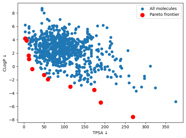
A small example of this uses the Caco2 dataset of small-molecule permeability from TDC. As in (Park et al. 2023), we compute some other molecular properties on this set using RDKit, and then illustrate the trade-offs among them by sketching out the Pareto frontier on this dataset with respect to these properties.

Following the prior work, the properties we compute for each molecule are ClogP (lipophilicity) and TPSA (topological polar surface area).

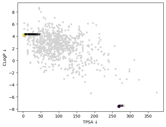
We extract the Pareto front, and visualize weighted‑sum and \(\epsilon\)‑constraint selections.

import pandas as pd
from rdkit import Chem
from rdkit.Chem import Descriptors
import matplotlib.pyplot as plt

def fetch_caco2():
    """
    Pull the full Caco-2 permeability set from TDC.
    """
    from tdc.single_pred import ADME
    data = ADME(name='Caco2_Wang')
    df = data.get_data()              # SMILES in 'SMILES', permeability in 'Y'
    return df[['Drug', 'Y']].rename(columns={'Drug': 'SMILES', 'Y': 'Permeability'})

def compute_props(df):
    clogp, tpsa, keep = [], [], []
    for idx, smi in df['SMILES'].items():
        mol = Chem.MolFromSmiles(smi)
        if mol is None:
            continue
        clogp.append(Descriptors.MolLogP(mol))
        tpsa.append(Descriptors.TPSA(mol))
        keep.append(idx)
    df = df.loc[keep].copy()
    df['CLogP'] = clogp
    df['TPSA']  = tpsa
    return df


df = compute_props(fetch_caco2())

Found local copy...
Loading...
Done!

props_names = ['TPSA', 'CLogP']
props_maximize = [False, False]

front = pareto_front(df[[props_names[0], props_names[1]]].values, maximize_array=props_maximize)
front_df = df[front]

# --- quick visual ----------------------------------------------------------
plt.clf()
plt.scatter(df[props_names[0]], df[props_names[1]], label='All molecules')
plt.scatter(front_df[props_names[0]], front_df[props_names[1]], s=90, c='red', label='Pareto frontier')
props_dirs = ['↑' if props_maximize[i] else '↓' for i in range(len(props_maximize))]

plt.xlabel(f"{props_names[0]} {props_dirs[0]}")
plt.ylabel(f"{props_names[1]} {props_dirs[1]}")
plt.legend()
plt.tight_layout()
plt.show()

# best = df.loc[(w*df['CLogP']-(1-w)*df['TPSA']).idxmax()]

weights = np.exp(np.linspace(-20, 20))
chosen = []

front = pareto_front(df[props_names].values, maximize_array=props_maximize)
front_df = df[front]

for w in weights:
    score = front_df[props_names[0]] + w*front_df[props_names[1]]
    idx = score.idxmax()
    chosen.append(idx)
    
chosen_df = df.loc[chosen].assign(w=weights)

fig, ax = plt.subplots()
ax.scatter(df[props_names[0]] , df[props_names[1]], c='lightgrey', s=12)
ax.scatter(chosen_df[props_names[0]] , chosen_df[props_names[1]],
           c=chosen_df.w, cmap='viridis', s=40, label='weight‑sum optima')
for _, r in chosen_df.iterrows():
    ax.text(r[props_names[0]], r[props_names[1]], f'{r.w:.1f}', fontsize=6)

props_dirs = ['↑' if props_maximize[i] else '↓' for i in range(len(props_maximize))]
ax.set_xlabel(f"{props_names[0]} {props_dirs[0]}")
ax.set_ylabel(f"{props_names[1]} {props_dirs[1]}")
plt.show()

ε‑constraint slice

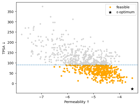
In this case, it’s reasonable to think of hard constraints on individual objectives. This is particularly the case in drug discovery, where such knowledge is often tacit and indirect. For instance, a reasonable constraint on TPSA is for it to be less than 90 square angstroms (Cornelissen et al. 2023), and for CLogp that it be less than 5, but also greater than -0.5. 

Such hard constraints are the other common way to formulate such problems. This can be easily implemented as below.

mask = df["TPSA"] <= 90
subset = df[mask]
best = subset['Permeability'].idxmax()

fig, ax = plt.subplots()
ax.scatter(df['Permeability'], df['TPSA'], c='lightgrey', s=12)
ax.axhline(90, ls='--', lw=1)
ax.scatter(subset['Permeability'], subset['TPSA'], c='orange', s=15, label='feasible')
ax.scatter(df.loc[best, 'Permeability'], -df.loc[best, 'TPSA'],
           c='black', s=60, marker='*', label='ε‑optimum')
ax.set_xlabel('Permeability ↑'); ax.set_ylabel('TPSA ↓')
ax.legend();
plt.show()

best = df.loc[(w*df['CLogP']-(1-w)*df['TPSA']).idxmax()]

Aside: explore–exploit bandits with multiple rewards

Multi‑objective regret minimization extends classic stochastic bandits:

\[ \text{regret}_T = \sum_{t\le T}\bigl( f(x^\star) - f(x_t) \bigr) \]

Algorithms like MO‑UCB maintain Pareto optimism sets.

Pragmatic guidelines

• The point we emphasize here is that taking linear combinations of individual objectives – the easy thing to do – is also principled and coherent, because it is equivalent to restricting the individual objectives.

• We always normalize objectives before scalarizing — otherwize the largest‑magnitude criterion dominates. A great standard solution is quantile normalization (i.e., representing each feature value with its percentile) with respect to a fixed reference distribution. This type of procedure plays very well with conformal confidence sets, which are widely utilized in multi-objective decision-making problems (Gruver et al. 2023). It has connections to multivariate ranks, which are a widely known algorithmic technique in MOO.

• Typically, it’s useful to think about surfacing several diverse Pareto points rather than forcing a single winner; humans like choice, and weights can and will be reassessed whenever business or scientific priorities shift.

Tacit information

There are other tacit ways to supply information into the multi-objective problem that really strongly dictate what the answer should be. Even among an informed group of stakeholders, weighing the objectives may be quite complicated in any absolute sense. But relative comparisons are often easier:

• Any information about rough marginal rates of substitution (“1 log‑unit potency is worth 0.3 log‑units toxicity in a particular part of solution space”) can be converted into weight ratios.

• Even binary “which one is better?” comparisons between pairs of objectives can be quickly converted into implied weights on the objectives. How this can be done efficiently is the subject of another post.

Why not Pareto?

Often, Pareto-frontier solutions are just guidelines for action, whether running an organization or discovering a drug. They are idealized ways to trade off many multiple objectives under uncertainty. The actions actually taken will often not be from the Pareto-optimal set, for various reasons.

One is indeterminacy: sometimes, the multiple objectives do not completely represent all the criteria used in arriving at a solution. When trying to implement solutions in the specific context of a project organization, unique project or organizational constraints are quite common. They are typically not encoded into the method, though they can be if they’re known beforehand.²

Another reason to deviate from Pareto optimality is hedging (“non-convexity”): sometimes, even hedging between different Pareto optimal solutions – not taking any of them, but rather a solution in between, or mixing several of them – does not lead to a Pareto optimal solution. In technical terms, this happens when the solution space or constraint set is not convex, which is the typical case in large-scale real-world applications such as molecular design.

Gradient-based methods

There’s a long tradition of gradient-based methods in learning under multiple objectives. The core quantitative tools again center around duality through weighted sums.

The duality around weighted sums, as we’ve outlined it above, has long been realized (Miettinen 1999). For some weights \(\lambda^*\) to be optimal here, they need to define a stationary point of the weighted-sum objective: \(\sum_{i} \lambda_{i}^* \nabla f_{i} (x) = 0\). This dual viewpoint underpins most modern gradient-based algorithms.

Deep multitask learning (MTL) trains one model on many objectives. Sener & Koltun (Sener and Koltun 2018) made the connection explicit: each task loss is an objective, and a descent direction satisfying Pareto KKT conditions ensures no task is sacrificed for another. Since that time, MOO theory has been popularized to design task-balancing optimizers.

MGDA (Minimum-norm Gradient Descent Algorithm) (Désidéri 2012) is another classic duality-based method. It attempts to find a direction to maximize the minimum decrease across all objectives. This can be further regularized by constraining the gradient to be close to some known direction. MGDA can be nudged towards a reference direction \(r\) by adding a regularization term \(\eta \| d - r \|^2\) has a dual form. The paper (Liu et al. 2021) gives another algorithm that adapts the dual form in a more aggressive way to ensure faster convergence - it chooses weights \(\lambda\) to shrink the largest cosine conflict between tasks, improving convergence speed.

There are many related papers on gradient-based MOO methods over the last few years, overviewed in some recent work (see e.g. (Xiao, Ban, and Ji 2023), (Chen et al. 2025)).

Summary

There is no single best answer in multi-criterion optimization problems, but we can easily find straightforward solutions to most of them in practice.

• Multi‑criterion spaces can be navigated by adapting single-criterion tools, with only a few lines of Python and a clear sense of priorities.

• Scalarization with weighted sums turns abstractions into implementable optimizations.

References

Chen, Weiyu, Baijiong Lin, Xiaoyuan Zhang, Xi Lin, Han Zhao, Qingfu Zhang, and James T Kwok. 2025. “Gradient-Based Multi-Objective Deep Learning: Algorithms, Theories, Applications, and Beyond.” arXiv Preprint arXiv:2501.10945.

Cornelissen, Fleur MG, Greta Markert, Ghislaine Deutsch, Maria Antonara, Noa Faaij, Imke Bartelink, David Noske, W Peter Vandertop, Andreas Bender, and Bart A Westerman. 2023. “Explaining Blood–Brain Barrier Permeability of Small Molecules by Integrated Analysis of Different Transport Mechanisms.” Journal of Medicinal Chemistry 66 (11): 7253–67.

Désidéri, Jean-Antoine. 2012. “Multiple-Gradient Descent Algorithm (MGDA) for Multiobjective Optimization.” Comptes Rendus Mathematique 350 (5-6): 313–18.

Gruver, Nate, Samuel Stanton, Nathan Frey, Tim GJ Rudner, Isidro Hotzel, Julien Lafrance-Vanasse, Arvind Rajpal, Kyunghyun Cho, and Andrew G Wilson. 2023. “Protein Design with Guided Discrete Diffusion.” Advances in Neural Information Processing Systems 36: 12489–517.

Lin, Xi, Zhiyuan Yang, Xiaoyuan Zhang, and Qingfu Zhang. 2022. “Pareto Set Learning for Expensive Multi-Objective Optimization.” Advances in Neural Information Processing Systems 35: 19231–47.

Liu, Bo, Xingchao Liu, Xiaojie Jin, Peter Stone, and Qiang Liu. 2021. “Conflict-Averse Gradient Descent for Multi-Task Learning.” Advances in Neural Information Processing Systems 34: 18878–90.

Mahapatra, Debabrata, and Vaibhav Rajan. 2020. “Multi-Task Learning with User Preferences: Gradient Descent with Controlled Ascent in Pareto Optimization.” In International Conference on Machine Learning, 6597–607. PMLR.

Miettinen, Kaisa. 1999. Nonlinear Multiobjective Optimization. Vol. 12. Springer Science & Business Media.

Navon, Aviv, Aviv Shamsian, Gal Chechik, and Ethan Fetaya. 2020. “Learning the Pareto Front with Hypernetworks.” arXiv Preprint arXiv:2010.04104.

Park, Ji Won, Nataša Tagasovska, Michael Maser, Stephen Ra, and Kyunghyun Cho. 2023. “BOtied: Multi-Objective Bayesian Optimization with Tied Multivariate Ranks.” arXiv Preprint arXiv:2306.00344.

Sener, Ozan, and Vladlen Koltun. 2018. “Multi-Task Learning as Multi-Objective Optimization.” Advances in Neural Information Processing Systems 31.

Sun, Duxin, Wei Gao, Hongxiang Hu, and Simon Zhou. 2022. “Why 90% of Clinical Drug Development Fails and How to Improve It?” Acta Pharmaceutica Sinica B 12 (7): 3049–62.

Xiao, Peiyao, Hao Ban, and Kaiyi Ji. 2023. “Direction-Oriented Multi-Objective Learning: Simple and Provable Stochastic Algorithms.” Advances in Neural Information Processing Systems 36: 4509–33.

Footnotes

1. This can be proved as a one-to-one correspondence.

2. Suppose, for instance, that there are a set of blacklisted design features in lead candidate molecules, for e.g. patent reasons. The set of blacklisted molecules would then be encoded as a new objective \(f(x) = \textbf{1} (x \in \text{blacklist})\), and this can be added into the objective function after being scaled by an accompanying regularization factor \(\lambda_{\text{blacklist}}\).